Anna M. Michałowska-Kaczmarczyk 1, Tadeusz Michałowski 2
1 Department of Oncology, The University Hospital in Cracow, 31-501 Cracow, Poland
2 Department of Analytical Chemistry, Technical University of Cracow, 31-155 Cracow, Poland
© 2019 Sift Desk Journals. All Rights Reserved
VOLUME: 2 ISSUE: 1
Page No: 88-113
Anna M. Michałowska-Kaczmarczyk 1, Tadeusz Michałowski 2
1 Department of Oncology, The University Hospital in Cracow, 31-501 Cracow, Poland
2 Department of Analytical Chemistry, Technical University of Cracow, 31-155 Cracow, Poland
Tadeusz Michalowski, The modified Gran methods in potentiometric redox titrations derived according to GATES/GEB principles(2018)Journal of Chemical Engineering And Bioanalytical Chemistry 2(1)
The paper concerns the modified Gran methods, designed for determination of equivalence volume (Veq) and the slope (J) value of a redox indicator electrode (RIE) applied for potentiometric titrations in redox systems. The methods are exemplified by the titration of (1o) FeSO4 and (2o) FeSO4 + Fe2(SO4)3 mixture with KMnO4 or Ce(SO4)2 solution as titrant. The modified Gran methods are based on detailed conclusions resulting from thermodynamic modelling of the related systems according to GATES/GEB principles.
Keywords: Redox titration; GATES/GEB; modified Gran methods; electrode calibration.
Notations and acronyms: D – titrand (solution titrated); E – voltage [V]; GATES – Generalized approach to electrolytic systems; GEB – Generalized electron balance; LSM – least squares method; T – titrant; V0 – volume [mL] of D; V – volume of T added into D from the start up to a given point of titration: T(V) ⟹ D(V0).
The original versions of the Gran I [1,2] and Gran II [3,4] methods, denoted later as G(I) and G(II) methods (for brevity), were designed for evaluation of equivalence volume (Veq) in potentiometric titrations, based on transformation of fragments of S-shaped titration curve into linear segments. Both methods, of extrapolative nature (extrapolative standard addition method), especially G(II) method, were widely exploited later in practice by chemists-analysts.
The progress in applications of the G(I) and G(II) methods for analytical purposes was not uniform when referred to the main areas of titrimetric analyses, i.e., acid-base, redox, complexation and precipitation titrations. The methods were devoted mainly to acid-base titration, with special emphasis put on alkalinity. As refers to redox systems, only a few papers of other authors were issued hitherto; all them were based on primitive models resulting from stoichiometry of redox reactions, where only the species entering the redox reaction notation were involved, see e.g. [5]. The functional dependencies based on those assumptions, gave erroneous experimental results for Veq, as were stated in [6-8], and confirmed later in the papers [9-12].
The modified Gran methods, based on the GATES/GEB [13-24] principles, will be illustrated on three examples of potentiometric redox titrations, T(V) ⟹ D(V0). The redox systems considered in this paper will be denoted as follows:
System I : KMnO4 (C) + CO2 (C2) ⟹ FeSO4 (C02) + H2SO4 (C04) + CO2 (C05) ,
System II : KMnO4 (C) + CO2 (C2) ⟹ FeSO4 (C02) + Fe2(SO4)3 (C03) + H2SO4 (C04) + CO2 (C05) ,
System III : Ce(SO4)2 (C) + H2SO4 (C1) + CO2 (C2) ⟹ FeSO4 (C02) + H2SO4 (C04) + CO2 (C05) ,
where C, C1, C2 and C02, C03, C04, C05 are concentrations [mol/L] of the corresponding solutes in T and D, respectively, completed by water. From formal viewpoint, the System I can be considered as a particular case of the System II, at C03 = 0. Some similarities inherent in the balances will be applied for further presentation of the balances in a compact form.
The detailed considerations regarding the modified Gran methods will be preceded by formulation of the Generalized Electron Balance (GEB) for the Systems II and III, according to the Approach II to GEB. The algebraic equivalency of Approaches I and II to GEB will also be proved.
The terms: components of the system and species in the system are distinguished. After mixing the components (solvent + solutes), a mixture of defined species is formed.
We refer here to aqueous electrolytic systems, where the species exist as hydrates , i=1,…, I; zi = 0, ±1, ±2,…is a charge, expressed in elementary charge units, e = F/NA (F = 96485 C∙mol−1 – Faraday’s constant, NA = 6.022∙1023 mol-1 – Avogadro’s number), ni = niW = niH2O ≥ 0 is a mean number of water (W=H2O) molecules attached to ; the case niW=0 is then also admitted.
For some reasons, it is justifiable to start the balancing from the numbers of particular entities: N0j – for components (j = 1,…,J) represented by molecules, and Ni – for the species (ions and molecules) of i-th kind (i = 1,…,I). The mono- or two-phase electrolytic system thus obtained involves N1 molecules of H2O and Ni species of i-th kind, (i=2, 3,…,I), specified briefly as (Ni, ni), where ni ≡ niW ≡ niH2O. For ordering purposes, we write: H+1 (N2, n2), OH-1 (N3, n3),…, where z2 = 1, z3 = –1,… .
The System II involves the non-redox subsystems:
(II.1) T(V) subsystem, composed of KMnO4 (N01) + H2O (N02) + CO2 (N03) ;
(II.2) D(V0) subsystem, composed of FeSO4∙7H2O (N04) + Fe2(SO4)3·xH2O (N05) + H2SO4 (N06) + H2O (N07) + CO2 (N08).
For I.2, we have N05 = 0 in the D(V0) subsystem.
The System III involves the non-redox subsystems:
(III.1) T(V) subsystem, composed of Ce(SO4)2∙4H2O (N01) + H2SO4 (N02) + H2O (N03) + CO2 (N04) ;
(III.2) D(V0) subsystem, composed of FeSO4∙7H2O (N05) + H2SO4 (N06) + H2O (N07) + CO2 (N08).
The common list of species, that will be applied/selected to particular Systems (I, II, III), is as follows:
H2O (N1); H+1 (N2, n2), OH-1 (N3, n3); HSO4-1 (N4, n4), SO4-2 (N5, n5); H2CO3 (N6, n6), HCO3-1 (N7, n7),
CO3-2 (N8, n8); Fe+2 (N9, n9), FeOH+1 (N10, n10), FeSO4 (N11, n11), Fe+3 (N12, n12), FeOH+2 (N13, n13),
Fe(OH)2+1 (N14, n14), Fe2(OH)2+4 (N15, n15); FeSO4+1 (N16, n16), Fe(SO4)2-1 (N17, n17); K+1 (N18, n18);
MnO4-1 (N19, n19), MnO4-2 (N20, n20), Mn+3 (N21, n21), MnOH+2 (N22, n22), Mn+2 (N23, n23),
MnOH+1 (N24, n24), MnSO4 (N25, n25); Ce+4 (N26, n26), CeOH+3 (N27, n27), Ce2(OH)3+5 (N28, n28),
Ce2(OH)4+4 (N29, n29), CeSO4+2 (N30, n30), Ce(SO4)2 (N31, n31), Ce(SO4)3-2 (N32, n32), Ce+3 (N33, n33),
CeOH+2 (N34, n34), CeSO4+1 (N35, n35), Ce(SO4)2-1 (N36, n36), Ce(SO4)3-3 (N37, n37).
The species, with the related ordinal numbers, will be applied in the balances, formulated below. Molar concentrations [mol/L] of the species are denoted as , for brevity.
The presence of carbonate species is considered here as an effect of CO2 from air, as the admixture of ‘pure’ water used on the step of D and T preparation; it may imitate the real conditions of the analysis, realised according to titrimetric mode.
The T and D can be considered as static (sub)systems of the dynamic D+T system realised in the titration T(V) ⟹ D(V0), where V mL of T is added into V0 mL of D, up to a defined point of the titration, and V0+V mL of D+T mixture is obtained at this point, if the additivity of the volumes is valid/tolerable. The D+T mixture is homogenized after each (small) consecutive portion of T added into D, to imitate the titration as the quasistatic process realised in a closed system, under isothermal conditions, pre-assumed for modelling purposes.
In aqueous media, we formulate charge balance, f0 = ChB, and elemental balances: f1 = f(H) for E1 = H (hydrogen) and f2 = f(O) for E2 = O (oxygen),… ; other elemental or core balances are denoted as fk = f(Yk), Yk = Ek or corek (k=3,…,K). A core is considered as a cluster of different atoms with defined composition (expressed by chemical formula), structure and external charge, unchanged in the system in question; e.g., SO4-2 is a core within the set of sulfate species: HSO4-1∙n4H2O, SO4-2 ∙n5H2O, FeSO4∙n11H2O in the (I.2) D(V0) subsystem.
In order to formulate the reliable (formally correct) set of balances for a given system, it is necessary to collect detailed, possibly complete (qualitative and quantitative) information regarding this system. The qualitative information concerns the components that make up the given system, and the species formed in this system. This information should subject thorough verification, when regarding the preparation of the appropriate solutions; e.g., Ce(SO4)2∙4H2O is dissolved in H2SO4 solution, not in water.
To avoid possible/simple mistakes in the realization of the linear combination procedure, we apply the equivalent relations:

for elements with negative oxidation numbers, or

for elements with positive oxidation numbers, k ∈ 3,…,K. In this notation, fk will be essentially treated not as the algebraic expression on the left side of the equation fk = 0, but as an equation that can be expressed in alternative forms presented above.
4. Formulation of balances for the System II
The balances are as follows:
f0 = ChB
N2 – N3 – N4 – 2N5 – N7 – 2N8 + 2N9 + N10 + 3N12 + 2N13 + N14 + 4N15 + N16 – N17 + N18 – N19 – 2N20 +
3N21 + 2N22 + 2N23 + N24 = 0 (1)
f1 = f(H)
2N1 + N2(1+2n2) + N3(1+2n3) + N4(1+2n4) + 2N5n5 + N6(2+2n6) + N7(1+2n7) + 2N8n8 + 2N9n9 +
N10(1+2n10) + 2N11n11 + 2N12n12 + N13(1+2n13) + N14(2+2n14) + N15(2+2n15) + 2N16n16 + 2N17n17 +
2N18n18 + 2N19n19 + 2N20n20 + 2N21n21 + N22(1+2n22) + 2N23n23 + N24(1+2n24) + 2N25n25
= 2N02 + 14N04 + 2xN05 + 2N06 + 2N07
f2 = f(O)
N1 + N2n2 + N3(1+n3) + N4(4+n4) + N5(4+n5) + N6(3+n6) + N7(3+n7) + N8(3+n8) + N9n9 +
N10(1+n10) + N11(4+n11) + N12n12 + N13(1+n13) + N14(2+n14) + N15(2+n15) + N16(4+n16) + N17(8+n17) +
N18n18 + N19(4+n19) + N20(4+n20) + N21n21 + N22(1+n22) + N23n23 + N24(1+n24) + N25(4+n25)
= 4N01 + N02 + 2N03 + 11N04 + (12+x)N05 + 4N06 + N07 + 2N08
–f3 = –f(SO4)
N04 + 3N05 + N06 = N4 + N5 + N11 + N16 + 2N17 + N25 (2)
–f4 = –f(CO3)
N03 + N08 = N6 + N7 + N8 (3)
–f5 = –f(Fe)
N04 + 2N05 = N9 + N10 + N11 + N12 + N13 + N14 + 2N15 + N16 + N17 (4)
–f6 = –f(K)
N01 = N18 (5)
–f7 = –f(Mn)
N01 = N19 + N20 + N21 + N22 + N23 + N24 + N25 (6)
f12 = 2∙f2 – f1
–N2 + N3 + 7N4 + 8N5 + 4N6 + 5N7 + 6N8 + N10 + 8N11 + N13 + 2N14 + 2N15 + 8N16 + 16N17 +
8N19 + 8N20 + N22 + N24 + 8N25 = 8N01 + 4N03 + 8N04 + 24N05 + 6N06 + 4N08 (7)
2∙f2 – f1 + f0 – 6f3 – 4f4 – f6 = 0 ⟺ (+1)∙f1 +(–2)∙f2 + (+6)∙f3 + (+4)∙f4 + (+1)∙f6 – f0 = 0 ⟺
(+1)∙f(H) + (–2)∙f(O) + (+6)∙f(SO4) + (+4)∙f(CO3) + (+1)∙f(K) – ChB = 0 (8)
2(N9+N10+N11) + 3(N12+N13+N14+2N15+N16+N17) + 7N19 + 6N20 + 3(N21+N22) + 2(N23+N24+N25)
= 7N01 + 2N04 + 6N05 (9)
Denoting the atomic numbers: ZFe = 26, ZMn = 25, from equations: 4, 6 and 9, we obtain the balance
ZFe∙f5 + ZMn∙f7 – (2∙f2 – f1 + f0 – 6f3 – 4f4 – f6)
(ZFe–2)(N9+N10+N11) + (ZFe–3)(N12+N13+N14+2N15+N16+N17) + (ZMn–7)N19 + (ZMn–6)N20 +
(ZMn–3)(N21+N22) + (ZMn–2)(N23+N24+N25) = (ZFe–2)N04 + 2(ZFe–3)N05 + (ZMn–7)N01 (10)
Next, we can apply the combination of equations 4, 6 and 10, giving the shortest form of GEB
3f5 + 2f7 – (2f2 – f1 + f0 – 6f3 – 4f4 – f6) = 0
(N9+N10+N11) – (5N19 + 4N20 + N21+N22) = N04 – 5N01 (11)
Applying the relations:
∙(V0+V) = 103∙ CV = 103∙N01/NA, C2V = 103∙N03/NA , C02V0 = 103∙N04/NA , C03V0 = 103∙N05/NA ,
C04V0 = 103∙N06/NA , C05V0 = 103∙N08/NA (12)
in the balances derived above, we have the optional/equivalent equations for GEB. From eq. 7, considered as the primary form of Generalized Electron Balance (GEB), f12 = pr-GEB, we obtain the equation
– [ H+1] + [OH-1] + 7[HSO4-1] + 8[SO4-2] + 4[H2CO3] + 5[HCO3-1] + 6[CO3-2] + [FeOH+1] +
8[FeSO4] + [FeOH+2] + 2[Fe(OH)2+1] + 2[Fe2(OH)2+4] + 8[FeSO4+1] + 16[Fe(SO4)2-1] +
8[MnO4-1] + 8[MnO4-2] + [MnOH+2] + [MnOH+1] + 8[MnSO4]
– (8CV + 4C2V + 8C02V0 + 24C03V0 + 6C04V0 + 4C05V0)/(V0+V) = 0 (7a)
Optionally, we have alternative forms of GEB for the System II:
2([Fe+2]+[FeOH+1]+[FeSO4]) + 3([Fe+3]+[FeOH+2]+[Fe(OH)2+1] +2[Fe2(OH)2+4]+[FeSO4+1]+
[Fe(SO4)2-1]) + 7[MnO4-1] + 6[MnO4-2] + 3([Mn+3]+[MnOH+2])
+ 2([Mn+2]+[MnOH+1]+[MnSO4]) – (2C0V0 +7CV)/(V0+V) = 0 (9a)
(ZFe–2)([Fe+2]+[FeOH+1]+[FeSO4]) + (ZFe–3)([Fe+3]+[FeOH+2]+[Fe(OH)2+1]+2[Fe2(OH)2+4] + [FeSO4+1]+[Fe(SO4)2-1]) + (ZMn–7)[MnO4-1] + (ZMn–6)[MnO4-2] + (ZMn–3)([Mn+3]+[MnOH+2]) +
(ZMn–2)([Mn+2]+[MnOH+1]+[MnSO4]) – ((ZFe–2)C0V0 + (ZMn–7)CV)/(V0+V) = 0 (10a)
[Fe+2]+[FeOH+1]+[FeSO4] – (5[MnO4-1] + 4[MnO4-2] + [Mn+3] + [MnOH+2])
– (C0V0 – 5CV)/(V0+V) = 0 (11a)
In other words, the GEB can be chosen arbitrarily from the set of equivalent equations: 7a, 9a, 10a, or 11a. The eq. 11a, as one of them, is completed by charge and concentration balances:
[H+1] – [OH-1] – [HSO4-1] – 2[SO4-2] – [HCO3-1] – 2[CO3-2] + 2[Fe+2] + [FeOH+1] + 3[Fe+3] + 2[FeOH+2] + [Fe(OH)2+1]+ 4[Fe2(OH)2+4] + [FeSO4+1] – [Fe(SO4)2-1] + [K+1] – [MnO4-1] – 2[MnO4-2]
+ 3[Mn+3] + 2[MnOH+2] + 2[Mn+2] + [MnOH+1] = 0 (1a)
[HSO4-1] + [SO4-2] + [FeSO4] + [FeSO4+1] + 2[Fe(SO4)2-1] + [MnSO4] – (C02+3C03+C04)V0/(V0+V) = 0 (2a)
[H2CO3] + [HCO3-1] + [CO3-2] – (C05V0+C2V)/(V0+V) = 0 (3a)
[Fe+2] + [FeOH+1] + [FeSO4] + [Fe+3] + [FeOH+2] + [Fe(OH)2+1] + 2[Fe2(OH)2+4] +
[FeSO4+1] + [Fe(SO4)2-1] – (C02+2C03)V0/(V0+V) = 0 (4a)
[K+1] = CV/(V0+V) (5a)
[MnO4-1] + [MnO4-2] + [Mn+3] + [MnOH+2] + [Mn+2] + [MnOH+1] + [MnSO4] – CV/(V0+V) = 0 (6a)
The relation (5a), where only one species is involved, is considered as equality, not equation.
The balances are as follows:
f0 = ChB
N2 – N3 – N4 – 2N5 – N7 – 2N8 + 2N9 + N10 + 3N12 + 2N13 + N14 + 4N15 + N16 – N17 + 4N18 +
3N19 + 5N20 + 4N21 + 2N22 – 2N24 + 3N25 + 2N26 + N27 – N28 – 3N29 = 0 (13)
f1 = f(H)
2N1 + N2(1+2n2) + N3(1+2n3) + N4(1+2n4) + 2N5n5 + N6(2+2n6) + N7(1+2n7) + 2N8n8 + 2N9n9 +
N10(1+2n10) + 2N11n11 + 2N12n12 + N13(1+2n13) + N14(2+2n14) + N15(2+2n15) + 2N16n16 + 2N17n17 +
2N26n26 + N27(1+2n27) + N28(3+2n28) + N29(4+2n29) + 2N30n30 + 2N31n31 + 2N32n32 + 2N33n33 +
N34(1+2n34) + 2N35n35 + 2N36n36 + 2N37n37 = 8N01 + 2N02 + 2N03 + 14N05 + 2N06 + 2N07
f2 = f(O)
N1 + N2n2 + N3(1+n3) + N4(4+n4) + N5(4+n5) + N6(3+n6) + N7(3+n7) + N8(3+n8) + N9n9 + N10(1+n10) +
N11(4+n11) + N12n12 + N13(1+n13) + N14(2+n14) + N15(2+n15) + N16(4+n16) + N17(8+n17) + N26n26 +
N27(1+n27) + N28(3+n28) + N29(4+n29) + N30(4+n30) + N31(8+n31) + N32(12+n32) + N33n33 + N34(1+n34) +
N35(4+n35) + N36(8+n36) + N37(12+n37) = 12N01 + 4N02 + N03 + 2N04 + 11N05 + 4N06 + N07 + 2N08
–f3 = –f(SO4)
2N01 + N02 + N05 + N06 = N4 + N5 + N11 + N16 + 2N17 + N30 + 2N31 + 3N32 + N35 + 2N36 + 3N37 (14)
–f4 = –f(CO3)
N04 + N08 = N6 + N7 + N8 (15)
–f5 = –f(Fe)
N05 = N9 + N10 + N11 + N12 + N13 + N14 + 2N15 + N16 + N17 (16)
–f6 = –f(Ce)
N01 = N26 + N27 + 2N28 + 2N29 + N30 + N31 + N32 + N33 + N34 + N35 + N36 + N37 (17)
f12 = 2∙f2 – f1
–N2 + N3 + 7N4 + 8N5 + 4N6 + 5N7 + 6N8 + N10 + 8N11 + N13 + 2N14 + 2N15 + 8N16 + 16N17 + N27 + 3N28 +
4N29 + 8N30 + 16N31 + 24N32 + N34 + 8N35 + 16N36 + 24N37 = 16N01 + 6N02 + 4N04 + 8N05 + 6N06 + 4N08 (18)
The linear combination
f12 + f0 – 6f3 – 4f4 = 0 ⟺ (+1)∙f1 + (–2)∙f2 + (+6)∙f3 + (+4)∙f4 – f0 = 0 ⟺
(+1)∙f(H) + (–2)∙f(O) + (+6)∙f(SO4) + (+4)∙f(CO3) – ChB = 0 (19)
involving K*=4 balances for electron-non-active elements: H, O, S, C (f(SO4) = f(S), f(CO3) = f(C)) gives the equation:
2(N9+N10+N11) + 3(N12+N13+N14+2N15+N16+N17) + 4(N26+N27+2N28+2N29+N30+N31+N32) +
3(N33+N34+N35+N36+N37) = 2N05 + 4N01 (20)
Denoting atomic numbers: ZFe = 26, ZCe = 58, from equations: 16, 17 and 20, we obtain the balance
ZFe∙f5 + ZCe∙f6 – (2∙f2 – f1 + f0 – 6f3 – 4f4)
(ZFe–2)∙(N9+N10+N11) + (ZFe–3)∙(N12+N13+N14+2N15+N16+N17) + (ZCe–4)∙(N26+N27+2N28+2N29+N30+N31+N32) + (ZCe–3)∙(N33+N34+N35+N36+N37) = (ZFe–2)∙N05 + (ZCe–4)∙N01 (21)
Applying the relations:
∙(V0+V) = 103∙, C02V0 = 103∙N01/NA, and CV = 103∙N05/NA (22)
in eq. 21, we obtain GEB, written in terms of molar concentrations
(ZFe–2)([Fe+2]+[FeOH+1]+[FeSO4]) + (ZFe–3)([Fe+3]+[FeOH+2]+[Fe(OH)2+1]+2[Fe2(OH)2+4]
+[FeSO4+1]+[Fe(SO4)2-1]) + (ZCe–4)([Ce+4]+[CeOH+3]+2[Ce2(OH)3+5] +2[Ce2(OH)4+4]+[CeSO4+2] +[Ce(SO4)2]+[Ce(SO4)3-2]) + (ZCe–3)([Ce+3]+[CeOH+2]+[CeSO4+1] +[Ce(SO4)2-1]+[Ce(SO4)3-3])
– ((ZFe–2)·C02V0 + (ZCe–4)·CV)/(V0+V) = 0 (21a)
Other linear combinations are also possible. Among others, we obtain the simpler form of GEB
3f5 + 3f6 – (f12 + f0 – 6f3 – 4f4) = 0
(N11+N12+N13) – (N21+N22+2N23+2N24+N25+N26+N27) = N01 – N05 ⟹ (23)
[Fe+2]+[FeOH+1]+[FeSO4] – ([Ce+4]+[CeOH+3]+2[Ce2(OH)3+5]+2[Ce2(OH)4+4]+
[CeSO4+2]+[Ce(SO4)2]+[Ce(SO4)3-2]) – (C02V0 – CV)/(V0+V) = 0 (23a)
From eq. 18, considered as the primary form of Generalized Electron Balance (GEB), f12 = pr-GEB, we obtain the equation
– [H+1] + [OH-1] + 7[HSO4-1] + 8[SO4-2] + 4[H2CO3] + 5[HCO3-1] + 6[CO3-2] + [FeOH+1] + 8[FeSO4] +
[FeOH+2] + 2[Fe(OH)2+1] + 2[Fe2(OH)2+4]+8[FeSO4+1]+16[Fe(SO4)2-1] + [CeOH+3] + 3[Ce2(OH)3+5] +
4[Ce2(OH)4+4] + 8[CeSO4+2] + 16[Ce(SO4)2] + 24[Ce(SO4)3-2] + [CeOH+2] + 8[CeSO4+1] +
16[Ce(SO4)2-1] + 24[Ce(SO4)3-3] – (16CV + 6(C01V0 + C1V) + 4(C02V0 + C2V))/(V0+V) = 0 (18a)
where, in addition to relations 22, we apply

From eq. 20 we have
2∙([Fe+2]+[FeOH+1]+[FeSO4]) + 3∙([Fe+3]+[FeOH+2]+[Fe(OH)2+1]+2[Fe2(OH)2+4]+[FeSO4+1]+[Fe(SO4)2-1]) + 4∙([Ce+4]+[CeOH+3]+2[Ce2(OH)3+5]+2[Ce2(OH)4+4]+[CeSO4+2] +[Ce(SO4)2]+[Ce(SO4)3-2]) + 3∙([Ce+3]+[CeOH+2]+[CeSO4+1]+[Ce(SO4)2-1]+[Ce(SO4)3-3]) – (2·C0V0 + 4·CV)/(V0+V) = 0 (20a)
The linear combination of equations: 16 (multiplied by 2), 17 (multiplied by 4) and 20 gives the next/shortest form of GEB
[Fe+3]+[FeOH+2]+[Fe(OH)2+1]+2[Fe2(OH)2+4]+[FeSO4+1]+[Fe(SO4)2-1] –
([Ce+3]+[CeOH+2]+[CeSO4+1]+[Ce(SO4)2-1]+[Ce(SO4)3-3]) = 0 (25)
where oxidized forms of Fe and reduced forms of Ce are interrelated; molar concentrations: C02 and C are not involved there explicitly.
For calculation purposes, related to the System III, the GEB, e.g. eq. 23a, is completed by charge and concentrations balances, obtained from equations 13-17 and relations 22, 24:
[H+1] – [OH-1] – [HSO4-1] – 2[SO4-2] – [HCO3-1] – 2[CO3-2] + 2[Fe+2] + [FeOH+1] +
3[Fe+3] + 2[FeOH+2] + [Fe(OH)2+1] + 4[Fe2(OH)2+4] + [FeSO4+1] – [Fe(SO4)2-1] +
4[Ce+4] + 3[CeOH+3] + 5[Ce2(OH)3+5] + 4[Ce2(OH)4+4] + 2[CeSO4+2] – 2[Ce(SO4)3-2] +
3[Ce+3] + 2[CeOH+2] + [CeSO4+1] – [Ce(SO4)2-1] – 3[Ce(SO4)3-3] = 0 (13a)
[HSO4-1] + [SO4-2] + [FeSO4] + [FeSO4+1] + 2[Fe(SO4)2-1] + [CeSO4+2] + 2[Ce(SO4)2] +
3[Ce(SO4)3-2] + [CeSO4+1] + 2[Ce(SO4)2-1] + 3[Ce(SO4)3-3] –
(C0V0 + C01V0 + 2CV + C1V)/(V0+V) = 0 (14a)
[H2CO3] + [HCO3-1] + [CO3-2] – (C02V0 + C2V)/(V0+V) = 0 (15a)
[Fe+2]+[FeOH+1]+[FeSO4] + [Fe+3]+[FeOH+2]+[Fe(OH)2+1]+2[Fe2(OH)2+4]+[FeSO4+1]+[Fe(SO4)2-1] – C02V0/(V0+V) = 0 (16a)
[Ce+4] + [CeOH+3] + 2[Ce2(OH)3+5] + 2[Ce2(OH)4+4] + [CeSO4+2] + [Ce(SO4)2] + [Ce(SO4)3-2] + [Ce+3] + [CeOH+2] + [CeSO4+1] + [Ce(SO4)2-1] + [Ce(SO4)3-3] – CV/(V0+V) = 0 (17a)
Concentrations of some species are interrelated in the set of independent expressions, where numerical values for the corresponding equilibrium constants are involved, and applied in the related algorithms.
[H+1][OH-1] = 10-14.0; [HSO4-1] = 101.8[H+1][SO4-2]; [H2CO3] = 1016.4[H+1]2[CO32]; [HCO3-1] = 1010.1[H+1][CO3-2];
[Fe+3] = [Fe+2]∙10A(E – 0.771); [FeOH+1] =104.5[Fe+2][OH-1]; [FeOH+2] = 1011.0[Fe+3][OH-1];
[Fe(OH)2+1] = 1021.7[Fe+3][OH-1]2; [Fe2(OH)2+4] = 1021.7[Fe+3]2[OH-1]2; [FeSO4] = 102.3[Fe+2][SO4-2];
[FeSO4+1] = 104.18[Fe+3][SO4-2]; [Fe(SO4)2-1] = 107.4[Fe+3][SO4-2]2;
[MnO4-1] = [Mn+2]∙105A(E – 1.507) + 8pH; [MnO4-2] = [Mn+2]∙104A(E – 1.743) + 8pH; [Mn+3] = [Mn+2]∙10A(E – 1.509);
[MnOH+2] = 1014.2[Mn+3][OH-1]; [MnSO4] = 102.28∙[Mn+2][SO4-2];
[Ce+4] = [Ce+3]∙10A(E–1.70); [CeOH+3] = 1013.3[Ce+4][OH-1]; [Ce2(OH)3+5] = 1013.3[Ce+4]2[OH-1]3;
[Ce2(OH)3+5] = 1040.3[Ce+4]2[OH-1]3; [Ce2(OH)4+4] = 1053.7[Ce+4]2[OH-1]4; [CeOH+2] = 105.0[Ce+3][OH-1]; [CeSO4+1] = 101.63[Ce+3][SO4-2]; [Ce(SO4)2-1] = 102.34[Ce+3][SO4-2]2; [Ce(SO4)3-3] = 103.08[Ce+3][SO4-2]3; [CeSO4+2] = 103.5[Ce+4][SO4-2]; [Ce(SO4)2] = 108.0[Ce+4][SO4-2]2; [Ce(SO4)3-2] = 1010.4[Ce+4][SO4-2]3. (26)
where

7. Fraction titrated
The results of simulated titrations, with measurable values: potential E and/or pH of the D+T system, are plotted as the functions E = E(V) and/or pH = pH(V). In some instances, it is more advantageous/reasonable to plot the graphs: E = E(Φ) and/or pH = pH(Φ), with the fraction titrated [25-28].

on the abscissa, where C0 – concentration [mol/L] of the analyte A in D, C – concentration [mol/L] of reagent B in T; V0 mL is the volume of D taken for titration, V is the current/total volume of T added into D from the start up to a given point/moment of the titration. The Φ provides a kind of uniformity/normalization of the related plots, i.e., independency on V0 value.
For the Systems I and III, where FeSO4 is the single analyte, eq. 28 can be rewritten as follows
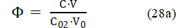
where C0 = C02.
The fraction titrated Φ (eq. 28) will be applied first to formulate the Generalized Equivalent Mass (GEM) concept.
8. Generalized equivalent mass (GEM)
The main task of a titration made for analytical purposes is the estimation of the equivalent volume, Veq, corresponding to the volume V of T, where the fraction titrated (eq. 28) assumes the value
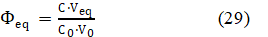
equal to the ratio p/q of small natural numbers p and q, Φeq = p/q. This ratio will be formulated on the basis of location of characteristic points on redox titration curves E = E(Φ).
In contradistinction to visual titrations, where the end (e) volume VeVeq is registered [21,27], all instrumental titrations aim, in principle, to obtain the Veq value on the basis of experimental data {(Vj, yj) | j=1,…,N}, where y = pH or E for potentiometric methods of analysis. Referring again to eq. 28, we have

where mA [g] and MA [g/mol] denote mass and molar mass of analyte (A), respectively. From equations: 28 and 30, we get

The value of the fraction in eq. 31, obtained from eq. 28,
is constant during the titration. Particularly, at the end (e) and equivalent (eq) points we have
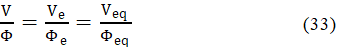
The Ve [mL] value is the volume of T consumed up to the end (e) point, where the titration is terminated (ended). The Ve value is usually determined in visual titration, when a pre-assumed color (or color change) of D+T mixture is obtained. In a visual acid-base titration, pHe value corresponds to the volume Ve [mL] of T added from the start of the titration, and
is the ɸ-value related to the end point. From equations 31 and 33, one obtains:

This does not mean, however, that we may choose between equations 35a and 35b, to calculate mA. Namely, eq. 35a cannot be applied for the evaluation of mA: Ve is known, but Fe is unknown; calculation of Fe needs prior knowledge of C0 value. However, C0 is unknown before the titration; otherwise, the titration would be purposeless. Also eq. 35b is useless: the ‘round’ Φeq value is known exactly, but Veq is unknown; Ve (not Veq) is determined in visual titrations.
Because the equations: 35a and 35b appear to be useless, the third, approximate formula for mA, has to be applied, namely:

where Φeq is put for Fe in eq. 35a, and
is named as the equivalent mass. The relative error in accuracy, resulting from this substitution, equals to

The Generalized Equivalence Mass (GEM) concept was formulated (1979) by Michałowski [18,19,21,25], as the counterproposal to earlier (1978) IUPAC decision [29], see also [30].
7. Computer program for the System I
The calculations in GATES/GEB are realized according to iterative computer program. The exemplary computer program, related to the System I, is as follows.
function F = Function_MnO4_Fe(x)
global V Vmin Vstep Vmax V0 C C2 C02 C04 C05 H OH fi pH E
global Kw pKw A K logK
global HSO4 SO4 logHSO4 logSO4
global H2CO3 HCO3 CO3 logH2CO3 logHCO3 logCO3
global Mn7O4 Mn6O4 Mn3 Mn3OH
global logMn7O4 logMn6O4 logMn3 logMn3OH
global Mn2 Mn2OH Mn2SO4
global logMn2 logMn2OH logMn2SO4
global Fe2 Fe2OH Fe2SO4
global logFe2 logFe2OH logFe2SO4
global Fe3 Fe3OH Fe3OH2 Fe32OH2 Fe3SO4 Fe3SO42
global logFe3 logFe3OH logFe3OH2 logFe32OH2 logFe3SO4 logFe3SO42
pH=x(1);
E=x(2);
Mn2=10.^-x(3);
Fe2=10.^-x(4);
SO4=10.^-x(5);
H2CO3=10.^-x(6);
H=10.^-pH;
pKw=14;
Kw=10.^-14;
OH=Kw./H;
A=16.9;
ZFe=26;
ZMn=25;
Mn7O4=Mn2.*10.^(5.*A.*(E-1.507)+8.*pH);
Mn6O4=Mn2.*10.^(4.*A.*(E-1.743)+8.*pH);
Mn3=Mn2.*10.^(A.*(E-1.509));
Fe3=Fe2.*10.^(A.*(E-0.771));
HSO4=10.^1.8.*H.*SO4;
HCO3=10.^(pH-6.3)*H2CO3.
CO3=10^(pH-10.1)*HCO3.
Fe2OH=10.^4.5.*Fe2.*OH;
Fe2SO4=10.^2.3.*Fe2.*SO4;
Fe3OH=10.^11.0.*Fe3.*OH;
Fe3OH2=10.^21.7.*Fe3.*OH.^2;
Fe32OH2=10.^25.1.*Fe3.^2.*OH.^2;
Fe3SO4=10.^4.18.*Fe3.*SO4;
Fe3SO42=10.^7.4.*Fe3.*SO4.^2;
Mn2OH=10.^3.4.*Mn2.*OH;
Mn2SO4=10.^2.28.*Mn2.*SO4;
Mn3OH=10.^14.2.*Mn3.*OH;
K=C.*V./(V0+V);
%Charge balance
F=[(H-OH+K-HSO4-HCO3-2.*CO3-2.*SO4-Mn7O4-2.*Mn6O4...
+3*Mn3+2.*Mn3OH+2.*Mn2+Mn2OH+2.*Fe2+Fe2OH+3.*Fe3...
+2.*Fe3OH+Fe3OH2+4.*Fe32OH2+Fe3SO4-Fe3SO42);
%Concentration balance of Mn
(Mn7O4+Mn6O4+Mn3+Mn3OH+Mn2+Mn2OH+Mn2SO4-C.*V./(V0+V));
%Concentration balance of Fe
(Fe2+Fe2OH+Fe2SO4+Fe3+Fe3OH+Fe3OH2+2.*Fe32OH2...
+Fe3SO4+Fe3SO42-C02.*V0./(V0+V));
%Concentration balance of S
(HSO4+SO4+Mn2SO4+Fe2SO4+Fe3SO4+2.*Fe3SO42...
-(C02+C04).*V0./(V0+V));
%Concentration balance of C
(H2CO3+HCO3+CO3-(C2*V+C05*V0)./(V0+V);
%Electron balance
((ZMn-7).*Mn7O4+(ZMn-6).*Mn6O4+(ZMn-3).*(Mn3+Mn3OH)...
+(ZMn-2).*(Mn2+Mn2OH+Mn2SO4)+(ZFe-2).*(Fe2+Fe2OH+Fe2SO4)...
+(ZFe-3).*(Fe3+Fe3OH+Fe3OH2+Fe32OH2+Fe3SO4+Fe3SO42)...
-((ZFe-2).*C02.*V0+(ZMn-7).*C.*V)./(V0+V))];
logMn2=log10(Mn2);
logMn2OH=log10(Mn2OH);
logMn2SO4=log10(Mn2SO4);
logMn3=log10(Mn3);
logMn3OH=log10(Mn3OH);
logMn6O4=log10(Mn6O4);
logMn7O4=log10(Mn7O4);
logFe2=log10(Fe2);
logFe2OH=log10(Fe2OH);
logFe2SO4=log10(Fe2SO4);
logFe3=log10(Fe3);
logFe3OH=log10(Fe3OH);
logFe3OH2=log10(Fe3OH2);
logFe32OH2=log10(Fe32OH2);
logFe3SO4=log10(Fe3SO4);
logFe3SO42=log10(Fe3SO42);
logHSO4=log10(HSO4);
logSO4=log10(SO4);
logH2CO3=log10(H2CO3);
logHCO3=log10(HCO3);
logCO3=log10(CO3);
logK=log10(K);
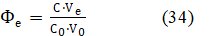
8. Graphical and numerical presentation of results
The results of calculations for the System I are presented graphically in Figures 1a-d, 2a-d (with E = E(Φ) and pH = pH(Φ) functions), and 3a,b, 4a,b (with speciation diagrams). Numerical data (Φ,E) from the vicinity of the jump in potential E-value (Fig. 1a) are collected in Table 1 [31]. The jump occurs here at Φ = Φeq = 0.2, named as equivalent (eq) point; note that 0.20000 ≡ ≡ 1 : 5. The coordinates of equivalent point are (Φeq, Eeq) = (0.20000, 1.034), with Φeq as the stoichiometric point of the reaction
MnO4-1 + 5Fe+2 + 8H+1 = Mn+2 + 5Fe+3 + 4H2O (39)
This reaction written in terms of predominating species (see Figures 3a,b) is as follows
MnO4-1 + 5FeSO4 + 6HSO4-1 + 2H+1 = MnSO4 + 5Fe(SO4)2-1 + 4H2O (40)
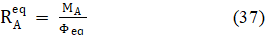
No changes in slope on the pH = pH(Φ) curves occur at Φeq = 0.2 (Fig. 1b), although one would expect, at first glance, that MnO4-1 may act, especially in reaction 39, like 'octopus' swallowing H+1 at Φ < 0.2, while the reaction 39 does not occur at Φ > 0.2. High value of the dynamic buffer capacity [32-34] in the D+T system is responsible for suppressing this effect. Analogous remark is related to the System III, represented by E = E(Φ) and pH = pH(Φ) relationships (Fig. 2), and speciation curves (Fig. 4).
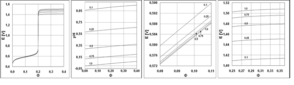
Fig. 1. The (1a) E = E(Φ) and (1b) pH = pH(Φ) curves plotted for the System I at V0 = 100, (C02,V0,C) = (0.01,100, 0.02) and different C04 values [mol/L], indicated in Figures 1b, 1c and 1d (in enlarged scales), before and after Φeq = 0.2; C2=C05=0.
Table 1. The pairs of (Φ, E) values for the System I, (C02,C04,V0,C) = (0.01,1.0,100, 0.02) in the close vicinity of (Φeq, Eeq); E in NHE scale
|
Φ |
E [V] |
|
0.19800 0.19900 0.19980 0.19990 0.19998 0.20000 0.20002 0.20010 0.20020 0.20200 |
0.701 0.719 0.761 0.778 0.820 1.034 1.323 1.365 1.382 1.442 |
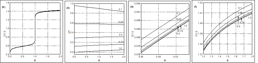
Fig. 2. The (2a) E = E(Φ) and (2b) pH = pH(Φ) curves plotted for the System III at V0 = 100, (C02,V0,C,C1) = (0.01,100, 0.1,1.0) and different C04 values [mol/L], indicated in Figures 2b, 2c and 2d (in enlarged scales), before and after Φeq = 1.0; C2=C05=0.
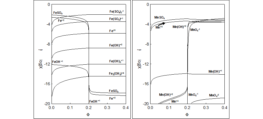
Fig. 3. Dynamic speciation diagrams for (3a) Fe-species, (3b) Mn-species in the System I ; (C02,C,C04) = (0.01,0.02,1.0), C2=C05=0, V0=100.
9. Formulation of the modified Gran methods
9.1. Preliminary relations
The redox potential E of a chemical system is measured with use of an inert metal (usually: platinum) as the indicator electrode in conjunction with a reference/counter electrode to form a complete cell; the E value in the system, involved with redox reaction
Fe+3 + e-1 = Fe+2 (41)
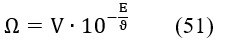
is expressed by the Nernst equation

where ϑ = a∙ln10 is the real slope of indicator electrode; and values are assumed constant during the titration; the involves standard redox potential E0 for reaction 41, potential of reference electrode, and liquid junction potential.
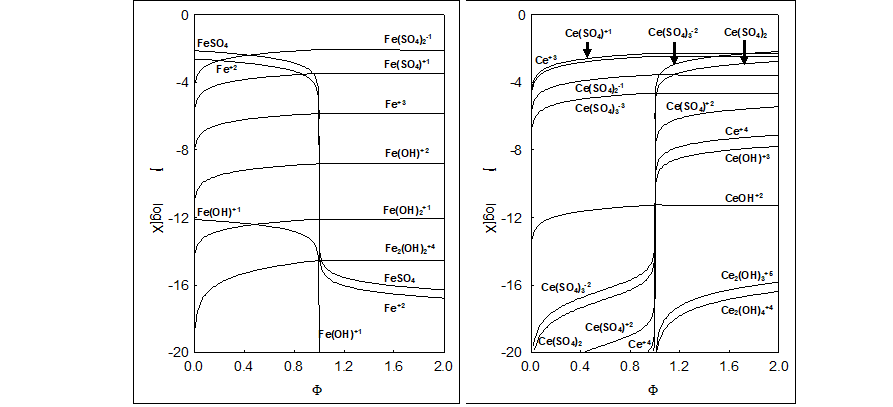
Fig.4. Dynamic speciation diagrams for (4a) Fe-species, (4b) Ce-species in the System III; (C,C1,C02,C04) = (0.1,0.5,0.02,1.0), C2=C05=0, V0=100.
For further discussion, we collect first the equations for GEB related to two different D+T systems: System I and System III, with FeSO4 (C02) + H2SO4 (C04) as D. The GEB expressed by eq. 11a, and rewritten as follows:
[Fe+2]+[FeOH+1]+[FeSO4] – (5[MnO4-1]+4[MnO4-2]+[Mn+3]+[MnOH+2]) = (C02V0 – 5CV)/(V0+V) (11b)
is applicable for the Systems I and II, whereas concentration balance for Fe in the System II is presented as follows
[Fe+2]+[FeOH+1]+[FeSO4] + [Fe+3]+[FeOH+2]+[Fe(OH)2+1]+2[Fe2(OH)2+4]+[FeSO4+1]+[Fe(SO4)2-1] = (C02+2C03)V0/(V0+V) (4b)
For the System I, we have C03=0 in eq. 4b, i.e.,
[Fe+2]+[FeOH+1]+[FeSO4]+[Fe+3]+[FeOH+2]+[Fe(OH)2+1]+2[Fe2(OH)2+4]+[FeSO4+1]+[Fe(SO4)2-1]= = C02V0/(V0+V) (4c)
In turn, for the System III we refer to equations 23a and 16a, rewritten analogously:
[Fe+2]+[FeOH+1]+[FeSO4] – ([Ce+4]+[CeOH+3]+2[Ce2(OH)3+5]+2[Ce2(OH)4+4]+ [CeSO4+2]+[Ce(SO4)2]+[Ce(SO4)3-2]) = (C02V0 – CV)/(V0+V) , and (23b)
[Fe+2]+[FeOH+1]+[FeSO4] + [Fe+3]+[FeOH+2]+[Fe(OH)2+1]+2[Fe2(OH)2+4]+[FeSO4+1]+[Fe(SO4)2-1] = C02V0/(V0+V) (16b)
The latter one is identical with eq. 4c.
9.2. Derivation of formulas for the Systems I and III
From relations: CV = Φ∙C02V0, and CVeq = Φeq∙C02V0, we have
At low pH values (Figures 1b, 2b), on the basis of speciation diagrams (Figures 3, 4), the balances: 11b and 23b at Φ < Φeq can be presented in the simplified forms:
[Fe+2] + [FeSO4] = (C02V0 – 5CV)/(V0+V) (at Φeq < 0.2, for the Systems I, II) (11c)
[Fe+2] + [FeSO4] = (C02V0 – CV)/(V0+V) (at Φeq < 1.0, for the System III) (23c)
At Φeq < 0.2 for the System I (Fig. 2) and at Φeq < 1.0 (Fig. 4) for the System III, the simplified balance for Fe can be applied
[Fe+2] + [FeSO4] + [Fe+3] + [FeSO4+1] + [Fe(SO4)2-1] = C02V0/(V0+V) (4c)
Applying the appropriate formulas found in (26), from equations: 11c, 23c and 4c we get, by turns:
[Fe+2]∙b2 = (C02V0 – 5CV)/(V0+V) (11d)
[Fe+2]∙b2 = (C02V0 – CV)/(V0+V) (23d)
[Fe+2]∙b2 + [Fe+3]∙b3 = C02V0/(V0+V) (4d)
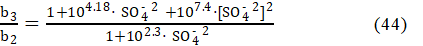
where : b2 = 1 + 102.3×[SO4–2] , b3 = 1 + 104.18×[SO4–2] + 107.4×[SO4–2]2, i.e.,

whereas from equations: 23d, 4d, 43 and Φeq =1, we have

i.e., the expressions for the ratio [Fe +3] /[Fe +2] are identical in the Systems: I and III. In the System III, the value of b3/b2 (eq. 44) depends on H2SO4 concentrations: C04 in D, and C1 in T, whereas in the System I, we have C1 = 0 in T. Then from equations: 42 and 45 (or 46), we get the relation

valid for V < Veq.
The θ = In b3/b2 vs. Φ relationships [10] are plotted for the Systems: I (Fig. 5a) and III (Fig. 5b). We see that dθ/dΦ <0 in Fig. 5a, and dθ/dΦ <0 in Fig. 5b. The θ vs. Φ relationships are quasi-linear, especially for greater C04 values. Then we can assume the relation


where ω = is the new constant value, obtained from constant values introduced above. From eq. 49 we have, by turns,

where ϑ = a∙ln10, and
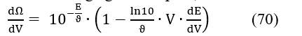
At high C04 value, the change of value is relatively small (Figures 5a,b); b = 1.7×10⁻³ at C04 = 1 mol/L. Then the assumption = const can be applied below in the simplified model. Putting β = 0 in eq. 50, we get

where G2 = = const. Applying in eq. 50 the approximation , valid for ≪ 1, we have, by turns
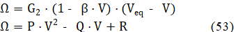
where:
P = G2∙β , Q = G2∙(β∙Veq + 1) , R = G2∙Veq (54)
Eq. 53 rewritten in the form of regression equation

is the basis for calculation of values for parameters: P, Q, R, determined according to the LSM. On the basis of relations 54, we get, by turns,

Equations 53a and 55 are the basis for the modified Gran II method in its accurate version, denoted in [ACA606] as MG(II)A, which improves the results dramatically. Moreover, the error z of analysis is not affected significantly by the true ϑ value for the slope of an indicator electrode.

Fig. 5. The q = ln(b3/b2) vs. F relationships for the Systems: I (5a), at (C,C02) = (0.02,0.01), and III (5b), plotted at (C,C1,C02) = (0.1,0.5,0.01), V0=100, C2=C05=0, and different C04 values indicated at the corresponding curves.
9.3. Accurate model
For two consecutive points (Vj, Ej) and (Vj+1, Ej+1) referred to potentiometric titration of D with T, from eq. 49 we have

Applying in eq. 56 the identities:
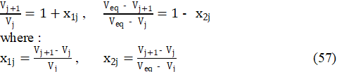
we get

Applying in eq. 52 the approximation [9-11,25,35] (see Fig. 6)

we write


where
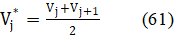

Fig. 6. Comparison of the plots for: (1) f1(x) = ln(1+x), (2) f2(x) = and (3) f3(x) = x, x ∈ < 0, 1 > .
Applying eq. 60b in eq. 58, we get the accurate model, written in terms of regression equation
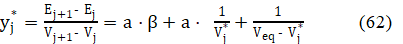
The parameters: Veq, a and β are obtained there according to an iterative computer program, by minimization of the sum of squares
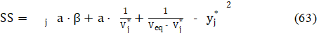
9.4. Approximate models (β=0)
Model 1.
Putting β = 0 in eq. 62, we get, after transformation
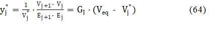
where
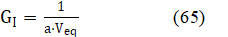
is a constant value, for the specific titration, see eq. 61. Denoting
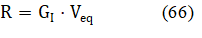
from eq. 58 we have the regression equation
The R and GI are determined there according to LSM:
and then we get
where 
in equations 68, 69; N – number of exp. points (Vj,Ej) | j=1,…,N. The formulation applied here is the basis for the modified G(I) method in its simplified version, denoted as MG(I)S version [10]. The great advantage of MG(I)S over G(I) method results from application of formulas 59 instead of approximation ln(1±x) ≈ ± x inherent in the G(I) method, see Fig. 6.
Model 2.
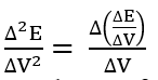
Referring again to eq. 52, we calculate the first and second derivatives of (eq. 51) [11]:

Note that the first derivative of eq. 52 is 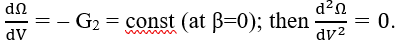
Zeroing the second derivative (eq. 71) gives
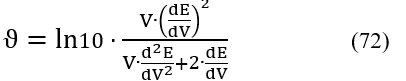
The first and second derivatives on the right side of Eq. 71 can be approximated by differential quotients
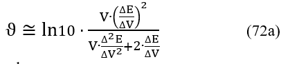
where
For the set of experimental points {(Vj, Ej)│j = 1,…, N – 1}, we have: ΔV = Vj+1 – Vj, ΔE = Ej+1 – Ej. Both differential quotients:
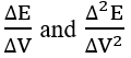
are put at Vj* (eq. 61). Then the Jj = J(Vj) values were calculated from the formula 72a. The formulas presented here are the basis for the MG(II)B method [11]. An alternative is here the MG(II)C method [11], based on the Lagrange polynomial interpolation method.
The interrelations between G(I), G(II) and different modifications of these methods are collected in [11].
9.5. Derivation of formulas for the System II
Referring to the System II, one can state/assume that the composition of the titrand D can be affected here by partial oxidation of the iron(+2) species by oxygen from air, as in the case of natural waters.
As stated above, eq. 11b and eq. 11d, as its simplified form, are valid also for the System II. At Φ < 0.2, the balance 4b can be written as follows

Then from equations 11d and 73 we get, by turns,

At C03=0, eq. 74 is transformed into equations 45, 46. From equations 42 and 74 we have

Assuming = const, i.e., β = 0 in eq. 48, and applying eq. 75 for two consecutive points (Vj, Ej) and (Vj+1, Ej+1) referred to potentiometric titration of D with T in the System II, we have
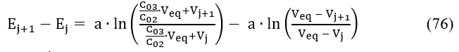
Denoting
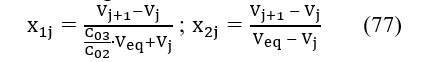
from eq. 76 we get

Applying the approximations 59 for 77, after transformations of eq. 76 we get, by turns,

and is the difference between the uj value found from measurements and the u() value found at V = from the model assumed. Then we calculate [9]

Calibration of redox indicator electrodes (RIEs) is of primary importance in potentiometric measurements performed in redox systems. The difficulties in calibration of RIEs were probably the main reason for generating the opinion on inapplicability of the Gran II (G(II)) method for determination of equivalence volume (Veq) in redox titrations. This problem has been exposed [10], where inaccuracy of the results obtained according to G(II) method at greater discrepancies between true (correct, J) and pre-assumed (Jc) slope values, |Jc – J| for RIEs has been proved [10]. It was also stated that the error in Veq can be substantially decreased, even at greater |Jc – J| values, if the modified Gran II method in its accurate version (MG(II)A) proposed in [10] is applied; the MG(II)A method improves the results dramatically (Fig. 7). The error z is not affected significantly by the true ϑ-value of an indicator electrode.
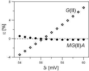
Fig. 7. The relationships between relative error e [%] in Veq determination vs J [mV] plotted for G(II) and MG(II)A methods, at Jc = 56 mV value pre-assumed in calculations [11].
It is stated that the linearizing approaches, inherent in original G(I) and G(II) methods, may provide inaccurate results of analyses. It were stated that the original Gran methods, particularly G(I) method [1], do not provide accurate results for Veq; the errors involved in G(I) may exceed tens percents, as indicated in [12]. Far more accurate results of analysis are obtainable according to the modified methods proposed by Michałowski in a series of papers [9-12,25], after recalling to the physicochemical nature of the system tested.
Also the original G(II) [3] method may not provide accurate results in the titrations; the matter lies in the divergence (ranging several percents [9]) between true and Nernstian slopes of the indicator electrode and in some difficulties encountered in calibration of this electrode.
In contradistinction to the G(II) method, the G(I) method offers the possibility to perform the potentiometric titrations without prior knowledge of ϑ – provided that ϑ is constant within defined V-range covered in the Gran methods, where the validity of assumption ϑ = ϑ(V) = const is increased – in contradistinction to the methods based on the inflection point location; a dramatic change of the analyte concentration occurs in the vicinity of this point. Such advantages of G(I) method were successfully exploited in the modified G(I) methods [9-12,25], thereafter referred to as simplified (MG(I)S) and accurate (MG(I)A) methods [10].
The results of calculations related to redox systems were obtained according to GATES/GEB principles, with use of the iterative computer program MATLAB and the generator of pseudo-random numbers [36]; these results were confirmed experimentally in [10,11].
The Generalized approach to electrolytic systems (GATES) [13] with the generalized electron balance (GEB) involved as GATES/GEB, is adaptable for resolution of thermodynamic (equilibrium and metastable) redox systems of any degree of complexity; none simplifying assumptions are needed [10]. Application of GATES provides the reference levels for real analytical systems, where some effects involved with kinetics and transportation (diffusion) phenomena occurred at the electrodes. The GATES makes possible to exhibit some important details, of qualitative and quantitative nature, invisible in real experiment, e.g. speciation. Reliability of physicochemical data (standard potentials, equilibrium constants of complexes, etc.) values is needed for this purpose. This requirement is fulfilled, among others, for 1◦ manganometric and 2◦ cerometric titrations of ferrous ions, where equilibria are established rapidly in the bulk solution. This way, we provide an approach to a more general problem involved with optimization a priori in redox systems, realized according to GATES principle.
The GATES approach is based on mathematical foundations, expressed by a system of nonlinear algebraic equations, not on a “fragile” chemical reaction notation, based on stoichiometry. Within GATES, the stoichiometry concept, as a resultant of all particular (stoichiometric, in principle) chemical reactions occurred in a dynamic system (as titration is) is not applied. Among others, the generalized equivalence mass (GEM) concept, based on GATES, is not involved with the stoichiometry concept. The stoichiometry is only a redundant concept within GATES and then formulation of reaction notation can be considered only as a kind of intellectual/didactic occupation, that can be made after presentation of the related curves obtained from calculations based on GATES.
The GEB (as Approaches I and II to GEB), GATES, GEM and all modifications of the Gran methods were discovered/suggested/formulated by Michałowski [9-12,25], and extended on different acid-base systems, involved also with total alkalinity [28,36,37], also with fulvic acids involved [38], and carbonate alkalinity [39], in particular.
Gran, G. (1950) Determination of the equivalence point in potentiometric titration, Acta Chemica Scandinavica 4 559-577. .
View ArticleGran, G. (1988) Equivalence volumes in potentiometric titrations, Analytica Chimica Acta 206: 111-123. 80835-1 ; https://www.sciencedirect.com/science/article/pii/S0003267000808351.
View ArticleGran, G. (1952) Determination of the equivalence point in potentiometric titrations. Part II, Analyst 77 661-671. .
View ArticleJohansson, A., Gran, G. (1980) Automatic titration by stepwise addition of equal volumes of titrant. Part V. Analyst, 105: 802-810.
View Articleda Conceição Silva Barreto, M., de Lucena Medeiros, L., César de Holanda Furtado, P. (2001) Indirect Potentiometric Titration of Fe(II) with Ce(IV) by Gran’s Method, Journal of Chemical Education 78: 91-92.
MacDonald, T.J., Barker, B.J., Caruso, J.A. (1972) Computer evaluation of titrations by Gran’s method. An analyti-cal chemistry experiment, Journal of Chemical Education, 49(3): 200-201.
Maccà, C., Bombi, G.G. (1989) Linearity range of Gran plots for the end-point in potentiometric titrations, Analyst, 114: 463-470.
Maccà, C. (1989) Linearity range of Gran plots from logarithmic diagrams, Analyst, 114: 689-694.
Michałowski, T., Baterowicz, A., Madej, A., Kochana, J. (2001) An extended Gran method and its applicability for simultaneous determination of Fe(II) and Fe(III), Analytica Chimica Acta 442(2): 287-293. .
View ArticleMichałowski, T., Kupiec, K., Rymanowski, M. (2008). Numerical analysis of the Gran methods. A comparative study, Analytica Chimica Acta 606(2): 172-183. http://suw.biblos.pk.edu.pl/resourceDetails&rId=4745%7D%7D%3C/opinion&rId=24153.
View ArticlePonikvar, M., Michałowski, T., Kupiec, K., Wybraniec, S., Rymanowski, M. (2008). Experimental verification of the modified Gran methods applicable to redox systems, Analytica Chimica Acta 628(2): 181-189. .
View ArticleMichałowski, T., Toporek, M., Rymanowski, M. (2005) Overview on the Gran and other linearization methods applied in titrimetric analyses, Talanta 65(5): 1241-1253. .
View ArticleT. Michałowski, Application of GATES and MATLAB for Resolution of Equilibrium, Metastable and Non-Equilibrium Electrolytic Systems, Chapter 1 (p. 1 – 34) in: Applications of MATLAB in Science and Engineering (ed. by T. Michałowski), InTech - Open Access publisher in the fields of Science, Technology and Medicine, 2011. ; http://cdn.intechweb.org/pdfs/18555.pdf
View ArticleMichałowski, T., Toporek, M., Michałowska-Kaczmarczyk, A.M., Asuero, A.G. (2013) New Trends in Studies on Electrolytic Redox Systems. Electrochimica Acta 109: 519–531.
View ArticleMichałowski, T., Michałowska-Kaczmarczyk, A.M., Toporek, M. (2013) Formulation of general criterion distin-guishing between non-redox and redox systems, Electrochimica Acta 112: 199-211. .
View ArticleMichałowska-Kaczmarczyk, A.M., Toporek, M., Michałowski, T. (2015) Speciation Diagrams in Dynamic Iodide + Dichromate System, Electrochimica Acta 155: 217–227.
View ArticleToporek, M., Michałowska-Kaczmarczyk, A.M., Michałowski, T. (2015) Symproportionation versus isproportionation in Bromine Redox Systems, Electrochimica Acta 171: 176–187.
View ArticleMichałowska-Kaczmarczyk, A.M., Asuero, A.G., Toporek, M., Michałowski, T. (2015) “Why not stoichiometry” versus “Stoichiometry – why not?” Part II. GATES in context with redox systems, Critical Reviews in Analytical Chemis-try 45(3): 240–268.
View ArticleMichałowska-Kaczmarczyk, A.M., Michałowski, T., Toporek, M., Asuero, A.G. (2015) “Why not stoichiometry” versus “Stoichiometry – why not?” Part III, Extension of GATES/GEB on Complex Dynamic Redox Systems, Critical Reviews in Analytical Chemistry, 45(4): 348-366.
View ArticleMichałowska-Kaczmarczyk, A.M., Spórna-Kucab, A., Michałowski, T. (2017) Generalized Electron Balance (GEB) as the Law of Nature in Electrolytic Redox Systems, in: Redox: Principles and Advanced Applications, Ali Khalid, M.A. (Ed.) InTech Chap. 2, 9-55. in https://www.intechopen.com/books/redox-principles-and-advanced-applications
View ArticleMichałowska-Kaczmarczyk, A.M., Spórna-Kucab, A., Michałowski, T. (2017) Principles of Titrimetric Analyses According to Generalized Approach to Electrolytic Systems (GATES), in: Advances in Titration Techniques, Vu Dang Hoang (Ed.), InTech Chap 5: 133-171. ; in: https://www.intechopen.com/books/advances-in-titration-techniques
View ArticleMichałowska-Kaczmarczyk, A.M., Spórna-Kucab, A., Michałowski, T. (2017) A Distinguishing Feature of the Balance 2∙f(O) – f(H) in Electrolytic Systems. The Reference to Titrimetric Methods of Analysis, in: Advances in Titra-tion Techniques. Vu Dang Hoang (Ed.), InTech Chap 6: 173-207. in https://www.intechopen.com/books/advances-in-titration-techniques
View ArticleMichałowska-Kaczmarczyk, A.M., Spórna-Kucab, A., Michałowski, T. (2017) Solubility products and solubility concepts, in: Descriptive Inorganic Chemistry. Researches of Metal Compounds. Akitsu T. (Ed.), InTech Chap 5: 93-134. in: https://www.intechopen.com/books/descriptive-inorganic-chemistry-researches-of-metal-compounds
View ArticleMichałowski T., Ponikvar-Svet, M., Asuero, A.G., Kupiec, K. (2012) Thermodynamic and kinetic effects involved with pH titration of As(III) with iodine in a buffered malonate system, Journal of Solution Chemistry 41(3): 436-446
View ArticleMichałowski T. (1981) Some remarks on acid-base titration curves, Chemia Analityczna 26: 799-813.
Michałowski, T. (2010) The Generalized Approach to Electrolytic Systems: I. Physicochemical and Analytical Im-plications, Critical Reviews in Analytical Chemistry, 40: 2-16.
View ArticleMichałowski, T., Pietrzyk, A., Ponikvar-Svet, M., Rymanowski, M. (2010) The Generalized Approach to Electrolyt-ic Systems: II. The Generalized Equivalent Mass (GEM) Concept, Critical Reviews in Analytical Chemistry 40: 17-29.
View ArticleAsuero, A.G., Michałowski, T. (2011) Comprehensive formulation of titration curves referred to complex acid-base systems and its analytical implications, Critical Reviews in Analytical Chemistry 41(2): 151-187. . http://www.tandfonline.com/doi/abs/10.1080/10408347.2011.559440
View ArticleWest, T.S. (1978) Recommendations on the usage of the terms ‘equivalent’ and ‘normal.’ Pure and Applied Chem-istry. 50: 325–338,
View ArticleZhao, M., Lu, I. (1994) abolition of the equivalent. Rule of equal amount of substance. Analytica Chimica Acta 289(1): 121–124.
Michałowski, T., Wajda, N., Janecki, D. (1996) A Unified Quantitative Approach to Electrolytic Systems, Chemia Analityczna (Warsaw), 41: 667-685. .
View ArticleMichałowska-Kaczmarczyk, A.M., Spórna-Kucab, A., Michałowski, T. (2017) Dynamic Buffer Capacities in Redox Systems, Journal of Chemistry and Applied Chemical Engineering, 1(2): 1 - 7 . . http://biochem-molbio.imedpub.com/dynamic-buffer-capacities-in-redox-systems.pdf.
View ArticleMichałowska-Kaczmarczyk, A.M., Michałowski, T. (2015) Dynamic Buffer Capacity in Acid-Base Systems, Jour-nal of Solution Chemistry, 44: 1256–1266. .
View ArticleMichałowska-Kaczmarczyk, A.M., Michałowski, T., Asuero, A.G. (2015) Formulation of dynamic buffer capacity for phytic acid, American Journal of Chemistry and Applications 2(1): 5-9.
View ArticleMichałowski, T., Stępak, R. (1985) Evaluation of the equivalence point in potentiometric titrations with application to traces of chloride, Analytica Chimica Acta, 172: 207-214.
MATLAB Function Reference, Version 7.0, The MathWorks Inc., .
View ArticleMichałowski, T., Asuero, A.G. (2012) New approaches in modelling the carbonate alkalinity and total alkalinity, Critical Reviews in Analytical Chemistry, 42: 220-244.
View ArticleMichałowska-Kaczmarczyk, A.M., Spórna-Kucab, A., Michałowski, T., Asuero, A.G. (2018) The Simms constants as parameters in hyperbolic functions related to acid-base titration curves, Journal of Chemistry and Applied Chemical Engineering, 2(2): 1-5.
View ArticleMichałowska-Kaczmarczyk, A.M., Michałowski, T. (2016) Application of Simms Constants in Modeling the Ti-trimetric Analyses of Fulvic Acids and Their Complexes with Metal Ions, Journal of Solution Chemistry 45: 200–220.
View ArticlePilarski, B., Michałowska-Kaczmarczyk, A.M., Asuero, A.G., Dobkowska, A., Lewandowska, M., Michałowski, T. (2014) A New Approach to Carbonate Alkalinity, Journal of Analytical Sciences, Methods and Instrumentation 4: 62-69.
View Article