Prof. Yejuan Wang
Email: wangyj@lzu.edu.cn
© 2019 Sift Desk Journals. All Rights Reserved
VOLUME: 5 ISSUE: 3
Page No: 90-102
Prof. Yejuan Wang
Email: wangyj@lzu.edu.cn
Tasir Khana, Naiming Yuanb,, Mian Gul Hilalc, Rafi Ullahd, Khan Alame, Muhammad Naveedf, Yejuan Wanga*
aSchool of Mathematics and Statistics, Gansu Key Laboratory of Applied Mathematics and Complex Systems, Lanzhou University, Lanzhou 730000, China
bCAS Key Laboratory of Regional Climate Environment for Temperate East Asia, Institute of Atmospheric Physics, Chinese Academy of Sciences, Beijing 100029, China
cMOE, Key laboratory of Cell activities and stress adaptations, School of life science, Lanzhou University, Lanzhou 730000, Gansu, PR China.
dState Key Laboratory of Grassland Agro‐ecosystems, Institute of Arid Agroecology, School of Life Sciences, Lanzhou University, Lanzhou 730000, China
eDepartment of Physics, University of Peshawar, Peshawar 25120, KPK, Pakistan
fInstitute of Microbiology, School of Life Sciences, Lanzhou University, Lanzhou 730000, Gansu, PR China.
Tasir Khan, Naiming Yuan, Mian Gul Hilal, Rafi Ullah, Khan Alam, Muhammad Naveed, Yejuan Wang. 2020: Frequency Analysis of Annual Maximum Temperature with Linear Moments for Parameter Estimation and Determination of Best Fit Probability Distribution for Regions in Pakistan. JESES, 5(3) ,pp: 90-102.
The evaluation of the annual maximum temperature (AMT) in different fields such as climatology, renewable energy and agricultural operation plays an important role in society. This study comprised of the frequency analysis of annual maximum temperature for eight sites in Pakistan, using multiple distribution techniques for a long period (1981-2016) with meteorological temperature data. Multiple parameter probability distributions (PDs), such as Generalized Normal, Generalized Extreme Value (GEV), Generalized Logistics (GLO), Generalized Pareto (GPA), Pearson type3, Log Pearson type3 and two parameter PDs, such as, Gumbel (GUM), Logistic (LOG), Normal and Log Normal were used to find the most suitable distribution for selected locations. The L-moments technique was used for the evaluation of distribution parameters of Anderson Darling test, Chi-square test and Kolmogorov Smirnov test. The L-moments ratio plot (L ratio plot) showed that three distributions; GPA, GEV and GLO were the best distributions for different stations and were better than the two parameter distribution.
Key words: Multiple Frequency analysis; Annual maximum temperature; L-moments; Pakistan
Temperature assessment plays a key role in studying the continuous change in the temperature rise or fall. A number of different works have been done on the climatic change in the environment, which conclude results on the crucial and complex rise and fall in temperature of the environment (Karpouzos et al., 2010; Cui et al., 2017). Studying the characteristics of precipitation change and regional temperature are particularly important for determining and understanding the impact of climate change in the atmospheric cycle, human society, ecological environment and agriculture. Climate warming affects precipitation characteristics, frequency and intensity. Since extreme temperature is associated with the most expensive and dangerous hazards, understanding the change and mechanism of extreme temperature in warming climate are of vital importance (Huang et al., 2019). In the events of climate change or global warming, slight changes in average temperature values can lead to significant changes in frequency and scale of extreme events, including extreme temperature (Yan et al., 2016).
Anomalies or extreme weather events are the main concern, as they have a significant human or economic impact. Climate warming caused by increasing concentration of greenhouse gases affects the social economic activity. For instance, lengthy heat waves and extremely high temperatures can challenge increasing water consumption, agricultural production and seriously effects on human health and even loss of life (Hasan et a.,2012). Climate change is diverse, ranging from droughts, floods, landslides, human health, endangered species, biodiversity, agricultural livelihoods and food security (Barnett, Adam and Lettenmaie, 2005). Humidity plays a vital role in the warming of the world temperature (Yang et al., 2012). In 2015 worldwide temperature almost terminates the conversation of hypothesized “global warming hiatus”, and the previous two warm years dismiss the discussion that increase in temperature was platitude. A close view shows a heating rate of the previous10 years is fewer than the past three decades (Schmidt, Shindell and Tsigaridis, 2014). Particularly the North Atlantic oscillation NAO has influence on the temperature where interior climate is in access. In the contest, the oceanic area climate is normalized, the outcome is weak or stimulates inconsequence (Bozyurt and Özdemir, 2014). The changing nature of extreme weather events around the world in the second half of the twentieth century are a general increase in warm nights, fewer days of frost, more frequent rainstorm events and lower frequencies of extreme low temperatures (Masud et al., 2016).
Changes in extreme events have enormous significances for world natural and human society. The intensity and frequency of extreme events may alter by climate change, and severe climate change can lead to more serious extreme events, with enormous influences and instable consequences. As a result, forecasting climate extremes is imperatively required to evaluate the influence of potential climate change on natural environment and human beings. Such indication is also hazardous for long-time planning of mitigation and adaptation strategies at the national and regional level (Frías et al., 2012). Extreme or irregular weather events are most important issues, as they have many socio-economic impacts (Hasan et al., 2012).
The increasing frequency of heat waves and the rapid melting of glaciers in northern Pakistan from 1985 to 2005 are the proofs of the strengthening trend of climate warming in the region (Rasul et al.,2008). The maximum increase in temperature had happened in the last 10 years. Temperature influences are responsible for changing the climate in Pakistan, for example; the heat waves have increased in each part of the l,. Accurate estimation of long-term trends in global and regional climate change is essential for attribution of impacts and forecast of climate change (Li, Dong and Jones, 2019). The effects of climate change, infrastructure and population continue to change in areas vulnerable to extreme effects such as floods, extreme temperatures and storm damage. In addition, land-use change often results in a greater vulnerability to extreme weather events, such as flooding caused by extreme rainfall events (Ozer and Mohamoud, 2013).
Non-parameter test is the best suitable model associated with data series to estimate the relationship between the observational frequency and the theoretical frequency. For temperature, the fit tests are the Chi-square test, Anderson Darling test and Kolmogorov Simon test can be highlighted (Sansigolo, 2008).
This work focuses on extreme temperatures in different locations of Pakistan. We emphasize the basic assumptions of stability, homogeneity and independence for maximum temperature frequency analysis (MTFA). These assumptions are significant before the MTFA, since the violation of these assumptions may result in misstatement of structural design estimates, due to which their actual use may become limited. Therefore, the main objectives of this work are in two aspects: (a) To present the best-fitted distribution and L-moments of the annual maximum temperature (AMT) series from eight meteorological stations from all the four provinces of Pakistan (Khyber Pakhtunkhwa, Sindh and Punjab of Pakistan); (b) The candidate distribution is evaluated using goodness of fit tests.
2.1. Weather observation sites of Pakistan
The climate in Pakistan has a lot of special and periodic changes. The most serious variables affecting the climate are humidity, temperature, wind speed and rainfall, some areas are deserts continue to be very dry and hot. Thirty-six years of data will be used to measure the probable trend of maximum temperature and annual average temperature. Eight stations from the major cities were selected from Pakistan meteorological department Islamabad. These stations are Astore, Peshawar, Lahore, Sialkot, Multan, Karachi, Hyderabad, and Quetta, and these sites are located in Khyber Pakhtunkhwa, Punjab, Sindh, and Baluchistan. The maximum temperature data achieved from Pakistan metrological department (PMD) Islamabad. The data of AMT from 1981 to 2016 will be analyzed in several decadal periods.
Karachi, the most populous city in Pakistan, is the capital of Sindh Province. Karachi is located southern Pakistan in Sindh province, and it is dry and pleasant compared to the hot season that began in March, and continues until the June monsoon. The Astor Valley is covered by approximately 250 square kilometers (97 square miles) of glaciers. The Astor Valley has a mild climate and in winter, the snow in the main valley can reach 6 inches (15 cm), however the snow in the mountains can reach 2-3 feet (60-90 cm). Multan, witnessed the most extreme temperatures in Pakistan, is located in the southern part of Punjab. Multan is in arid climate hot summers and cold winters. Summer begins in May and lasts until September. Summer is the longest season in Multan and heavy rain will occur during the monsoon season. Quetta, located in the northern part of Baluchistan province, is the capital and largest city of Baluchistan Province in Pakistan. Quetta, close to the Pakistan-Afghanistan border, is a semi-arid climate with very different temperatures between summer and winter. Summer begins in late May and lasts until the beginning of September, and the fall is from late September to mid-November. Winter begins in late November and ends in late March, while spring lasts from early April to late May. There is no heavy rain during the monsoon season in Quetta. Peshawar, close to the eastern end of the historic Khyber Pass and the Afghan border, is the capital city of Khyber Pakhtunkhwa. Affected by the local grassland climate, Peshawar has a semi-arid and hot climate with hot summers and mild winters. Unlike other parts of Pakistan, Peshawar is not a monsoon area. Lahore, the largest city and historical and cultural center in the Punjab region. The climate in Lahore is semi-arid. The rainy season start from late June, the rainiest month is July and the coolest month is January. Sialkot in northwest Panjab is located. It has four sub-seasonal moist subtropical features. The weather in Sialkot is still hot during the day, but it is cool at night with low humidity. In winter, the weather is slightly warmer and heavy precipitation. In this paper, all of the above eight cities will be used to represent maximum temperature characteristics. The annual maximum temperature series from Astor, Karachi, Hyderabad, Quetta, Lahore, Sialkot, Multan and Peshawar weather stations were collected by the PMD Islamabad. The location of annual maximum temperature is given in Fig. 1.
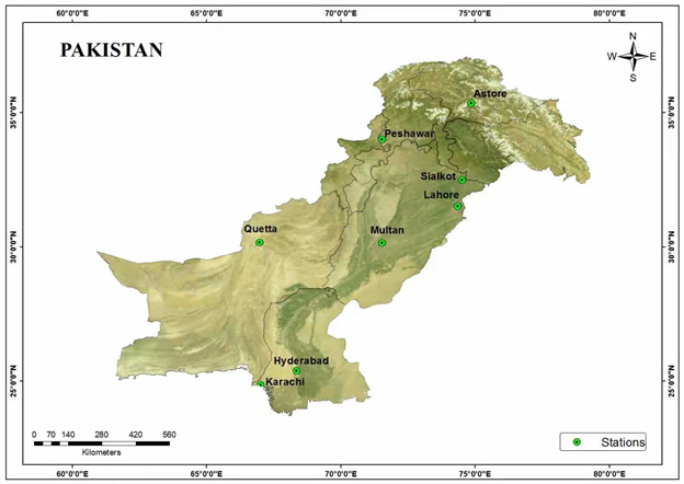
Fig. 1. Map and location of eight selected stations in Pakistan
Table.1 list of statistics for each site containing kurtosis, skewness, mean, altitude, latitude and longitude. The AMT series are thirty six years. The mean temperature between 27.65 and 41.43. The skewness of the Karachi station is greater than 1, which can be considered as a high degree of skewness. The skewness of the remaining stations ranges from -0.61 to 0.11 and can considered as approximately asymmetric to symmetric. As we can see from Table 1, the maximum temperature is 29.70 to 44.10. The latitude of the station is 24°54' to 32°30' north latitude and 67°0' to 81°31' east longitude. Altitude is an important factor in explaining extreme temperatures, which the temperature below at higher altitudes due to reduced. The elevation ranges from 4 meter to 2600 meter. Among all stations, the Astore station 2600 meter high is the highest elevation, while the Quetta station 1589 meter high is near to the Astore station in positions of height. In addition, the Karachi station four mete high has the bottom altitude. The lowest average temperature occurs at the highest altitude Astore station. However, the average temperature at the Karachi station at low altitude (4 m) is lower. This suggests that various other factors also affect temperature, making it challenging to find the association between simple average and geographical features. Therefore it is compulsory to study the influence of other aspects, such as large scale and small scale features , Therefore, it is compulsory to study the influence of other aspects, such as large-scale and small-scale features, topographical features, the presence of surface roughness, obstacles and ridge depressions in the main areas.
2.2. Preliminary analysis of annual maximum temperature
Prior to frequency analysis, annual maximum temperature sequence must satisfy specific statistical conditions such as homogeneity, independent and stationarity. For frequency analysis in extreme events, like extreme rainfall, extreme temperature and floods, these are common assumptions. The Augmented Dickey fuller test, Mann Kendall test, Mann-Whitney U test and Wald-Wolfowitz test could be applied to AMT series to check trend, homogeneity, stationarity, and independence.
2.2.1. Mann Kendall (MK) test
The nonparametric Mann Kendall test (Mann, 1945; Kendall, 1975; Gilbert, 1987) commonly used to examine monotonic patterns of decreasing or increasing trends in the data being studied. It shows that the trend is negative or positive. There is no monotonic trend in temperature sequence for null hypothesis Ho Mann- Kendall test, the random variable tp is independent identically distributed. The MK test statistics is as follows:
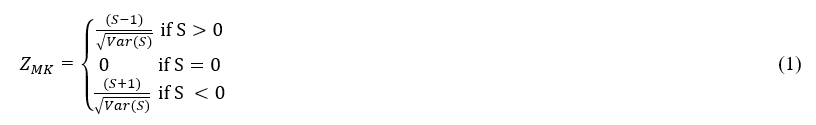
Where

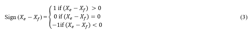

Where xe and xf are the value in time f and e, separately. In the data set g denote the different numbers of groups and tp represent data points in the pth binding groups. If n>8 then the statistics S follows the normal distribution. When ZMK≥Z1-α⁄2 the Ho do not accept.
2.2.2. Augmented Dickey Fuller (ADF) test
The augmented Dickey Fuller test was established by Dickey and Fuller (1979) and is usually used to check the stationary sequence. In the ADF test, the variables studied follow an autoregressive process. Compared with the original DF test, the ADF test can provide a higher order correlation parametric correction. The ADF test useful to more intricate time series models. The first-order autoregressive process of the DF test is as follow:
![]()
Autoregressive parameter is ρ and εt is the random component of the model. In case H0:ρ=1, the sequence is a unit root test, and thus the variable under study, represented as I(1), is non-stationary. For another case H1:|ρ|<1, the series, represented as I(0), does not contain a unit root, which shows that the sequence is stationary. To estimate DF test, by subtracting yt-1 from both sides of Eq. (5) we have
![]()
Where β=ρ-1 . The DF test statistic is defined by

In Eq. (7), ρ' is an estimate of , ρ and S'ρ is the estimated standard error of ρ'. Under H0, tDF follows the DF distribution. The critical value of the DF distribution has been given in {Dickey, 1976 #20} and {Fuller, 1976 #19}. By using linear trend, Dickey and fuller extended Eq. (5) as follows:
![]()
![]()
If the casual factor of Dicky Fuller model is auto correlated, then Eq. (5) revised as

The ADF test is given by
![]()
A real problem associated with ADF test (Schwert, 2002) suggested that the maximum pmax=12(T/100) the test effect on autocorrelation when p is very small and the test will be less effective when p is large. By linear trend its follow from Eq. (10) that
![]()
Where

Here dt is the deterministic term in Eq. (12).
2.2.3. Wald-Wolfowitz (WW) test for independence
The assumption of independence usually verified for hydrological variable, for instance annual average maximum or minimum, monthly, seasonal and other extreme data sample. The WW test originally suggested by Wald and Wolfowitz (1943) is often used to check the independence of the observational series (Naghettini, 2017; Surampalli, 2013). The WW test also can be used to check the existence of data trends. Let x1,x2,x3,....,xn be the observed value. Then Q statistics as given (Hamed and Rao, 1999).

The normal distribution Q statistic with mean and variance as follows


Here Sq = nm'q and m'q is the moments relative to the origin of the sample. The test statistic as

To check the independence at the significance level α for data sets. If the scale of statistic R is less than standard normal Rα⁄2 corresponding to the excess probability α⁄2, then H0 is accepted, its mean that the variable studied are independent.
2.2.4. Mann-Whitney U (MWU) test
The Mann Whitney U test, established by Mann and Whitney (1947), is a nonparametric test to check whether two samples come from the same population or not. When the data violates the normality assumption, the MWU test can replace the t test. It is also U test, is usually used to test the homogeneity assumption for frequency analysis of extreme events. Set p and q two sample size with p ≤ q. Let N = p +q be the total number of sample size; all sample are arranged in ascending order. The test depends on minimum "U" defined by (Naghettini, 2017; Mann, 1947).
![]()
![]()
![]()
Here p and q, respectively, denote the first and second samples sizes; where Y=∑ni=1Ri where Ri is the rank of the 1st sample p. denote by V the number of times, the p component follows first sample and q follows second in a similar way. The U statistics is defined by


In the occurrence parallel ranks, the variance formula of U should be rewritten as

Where Ji represents the observations rank k and i is the number of similar ranks.
2.3. Candidate probability distributions (PDs)
In this study two parameters distribution and seven multi parameter distributions, used commonly in frequency analysis of extreme event, will be used for maximum temperature frequency analysis (MTFA). These distributions are Gumbel (GUM), Logical (LOG), Normal (NOR), Generalized Logistic (GLO), generalized extreme value (GEV), generalize normal (GNO), generalized Pareto (GPA), Pearson Type 3 (PE3), Log Pearson type 3 (LP3), Log Normal (LN), Normal (NOR). Mostly distribution proposed on-site temperature and wind temperature analysis (Senapeng, 2017; Rajabi, 2008).
2.4. The method of L-moments estimation parameters of PDs
In current work, the L moment method used in extreme temperature used frequency analysis will be chose to estimate the parameters. This technique was suggested by Hosking and Wallis (2005), is a linear combination of sequential statistics ranked in descending or ascending direction. Linear moments are more consistent, since in outliers it is less sensitive. Compare with the maximum likelihood method, the method of moments and linear moments is appropriate for a small sample size (Hosking, 1987; Hosking, 1990; Alam, 2016). The linear moments also communicated in the sense of probability weighted moments (PWM).

Here r=1,2 3,….
The L-moments λr+1 can be given as follows:
![]()

The first four overall L-moments (λ1,λ2,λ3,λ4) involving position, ratio, L- kurtosis and L- skewness respectively, can be defined by
![]()
![]()
![]()
![]()

![]()

br, usually used in practice, is an unbiased estimator of βr

The relation of the first four sample L-moments with probability weighted moments are stated as follows
![]()
![]()
![]()
![]()
The sample L-ratios are

Where t is the measure of L-CV, t3 and t4, respectively, are the L- kurtosis and L- skewness of the sample?
2.5. Goodness of fit test
The special PD is affected by some aspects, such as comparison of probability distributions, the availability of maximum temperature data and the method of parameter estimation. In this work, the Anderson Darling test, Kolmogorov Smirnov and χ2 test difference criteria will be used for evaluating the suitability of different PDs. The difference between theoretical value and actual data sequence can be provided by goodness of fit tests. In order to check the visual evaluation of the fitness, we will make Quantile-Quantile (Q-Q) plots, L-moment ratio, extreme value and probability plots. The advantage of the above graphical test and fit test have been applied to maximum temperature data (Kunz et al. 2010; Yuan, 2018; Lawan, 2015).
2.5.1. Kolmogorov Smirnov (KS) test
The KS test is often adopted on the bases on empirical distribution function, the sample come from hypothetical continuous distribution. A random sample assume that there is x1,x2,x3,....,xn from some distribution. Then the EDF can be defined by

The Kolmogorov Smirnov statistic, depending on the maximum perpendicular distance between the EDF and the theoretical PD, is given as follow

In equation (44), F(xi) is the cumulative distribution function, xi is the ith order statistic and n denotes the sample size.
2.5.2. Anderson-Darling (AD) test
The test can be used to compare the fit of observed and theoretical distribution functions. The Anderson Darling test allocates a larger weight to the tail of the distribution, which is a fundamental feature of modeling extreme events (Huang et al. 2018). The AD test statistic A2 can be defined by

Here A2 is associated to the test outcome. the sample size n, the variable X and the distribution function, F(xi)
2.5.3. The Chi-square (χ2) test
Suppose that A1,A2,…,Ar denote a collection of detailed disjoint events, which can be combined to define the entire sample space. We also assume that the null hypothesis Ho: {P(Ai)=pi,and for i=1,2,3……,r} so that . In addition, it is assumed that the absolute frequency associated with A1,A2,…,Ar is given by the measures separately from N number of random experiments (Sansigolo, 2008). If Ho is true, then the joint probability distribution function associated with the variables ρ1,ρ2,…,ρr is

Where ∑r(i=1)Oi =N
The χ2 test statistic is given by
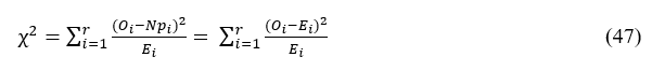
Where the expected value Ei:=E(ρi), is equal to NPi under Ho. Thus the χ2 statistic represents the sum of squared differences between the implementation of the random variables ρi and their respective expected values.
Frequency analysis is the first step to check the homogeneity, independence and stationarity of AMT series. Excluding random variations, stationarity means that series of annual maximum temperature is invariant with respect to time. Non-stationary is characterized by trends, jumping and looping. Regular changes in temperature the climate condition may result in trends, while long-term climate fluctuation leads to cycles. The abrupt variation in the river jumps mainly occur in flood frequency. Independence mean that the sequence observation has no effect on any other observation. In fact, the dependence may vary with interval length between consecutive elements of the sequence. However, for daily values it is often powerful. The homogeneity means that all observation data come from the same population. If the variation of extreme events (temperature, flood, rainfall and snowmelt) is rather large, then the homogeneity trend is too hard to interpret. But in this case, it can be considered as uniform because of the outcome of the test. On the other hand, heterogeneity is easier to identify from annual series.
The Augmented Dickey Fuller test, Mann-Whitney U (MWU), Mann Kendall (MK), Augmented Dickey Fuller (ADF) and Wald-Wolfowitz (WW) test, have be performed to check the trend, stationarity, homogeneity and independence. All the annual maximum temperature (AMT) series from eight stations approved all of the tests at 95% level of significance. The results of ADF, MWU, WW and MK test are present in Table 2. When these rules about the annual maximum temperature series not full fill, then you must adopt more complicated statistical methods to investigate the relationship between the observed data and their variation over the time. The time series plots of eight sites are described in Figure 2. In addition to finding monotonic trends, Figure 2 shows that MK test results are consistent with time series plots.
Table 1. Descriptive statistics of eight stations
|
Variable |
SD |
Skewness |
Kurtosis |
Mean |
Max Temp |
Latitude |
Longitude |
Altitude (m) |
|
Astore |
1.24 |
-0.61 |
1.05 |
27.65 |
29.70 |
29°9' |
81°31' |
2600 |
|
Karachi |
0.76 |
1.08 |
4.16 |
36.27 |
39 |
24°54' |
67°4' |
4 |
|
Hyderabad |
0.78 |
0.03 |
0.14 |
41.43 |
43.10 |
25°23' |
68°22' |
7 |
|
Quetta |
0.81 |
0.11 |
-1.16 |
36.71 |
38.30 |
30°11' |
67°0' |
1589 |
|
Lahore |
1.25 |
-0.46 |
1.25 |
40.22 |
43.10 |
31°33' |
74°19' |
215 |
|
Sialkot |
1.55 |
-0.14 |
-0.30 |
40.09 |
43.23 |
32°30' |
74°31' |
256 |
|
Multan |
1.06 |
-0.26 |
-0.61 |
42.43 |
44.10 |
30°11' |
71°28' |
123 |
|
Peshawar |
1.33 |
0.07 |
-0.43 |
40.12 |
42.70 |
34°0' |
71°35' |
359 |
Table 2. Testing the assumptions of independence, stationarity, and homogeneity of annual maximum temperature sequence of eight stations.
|
Station |
MK test |
ADF test |
WW test |
MWU test |
|||||||
|
TS |
P-value |
TS |
P-value |
TS |
P-value |
TS |
P-value |
||||
|
Astore |
-0.036 |
0.764 |
-6.175 |
0.0000 |
-0.1818 |
0.4279 |
-0.5695 |
0.2845 |
|||
|
Karachi |
0.152 |
0.203 |
-4.913 |
0.0003 |
1.9838 |
0.0236 |
-0.791 |
0.2145 |
|||
|
Hyderabad |
-0.159 |
0.181 |
5.149 |
0.0002 |
0.8164 |
0.2071 |
-1.4237 |
0.0773 |
|||
|
Quetta |
0.386 |
0.001 |
-4.286 |
0.0018 |
1.1626 |
0.125 |
-2.4994 |
0.0062 |
|||
|
Lahore |
-0.140 |
0.240 |
4.685 |
0.0006 |
1.5361 |
0.0623 |
-1.5503 |
0.0605 |
|||
|
Sialkot |
-0.282 |
0.016 |
3.783 |
0.0061 |
1.0904 |
0.183 |
-1.3605 |
0.2860 |
|||
|
Multan |
0.244 |
0.038 |
4.614 |
0.0007 |
1.6242 |
0.0522 |
-1.2972 |
0.0973 |
|||
|
Peshawar |
-0.338 |
0.004 |
-4.984 |
0.0031 |
1.0243 |
0.1528 |
-2.3413 |
0.0960 |
|||
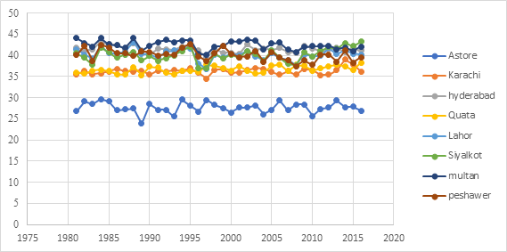
Fig. 2. Time series plots for eight stations
3.1. Probability distribution function (PDF)
Using PD analysis, the maximum temperature for selected all stations is calculated by means of several PDFs. Figure 3 displays the PD analysis of data series for representative stations (Astore, Karachi, Hyderabad, Quetta, Lahore, Sialkot, Multan, and Peshawar) are different regions and displays the result of probability distribution are different for every station.
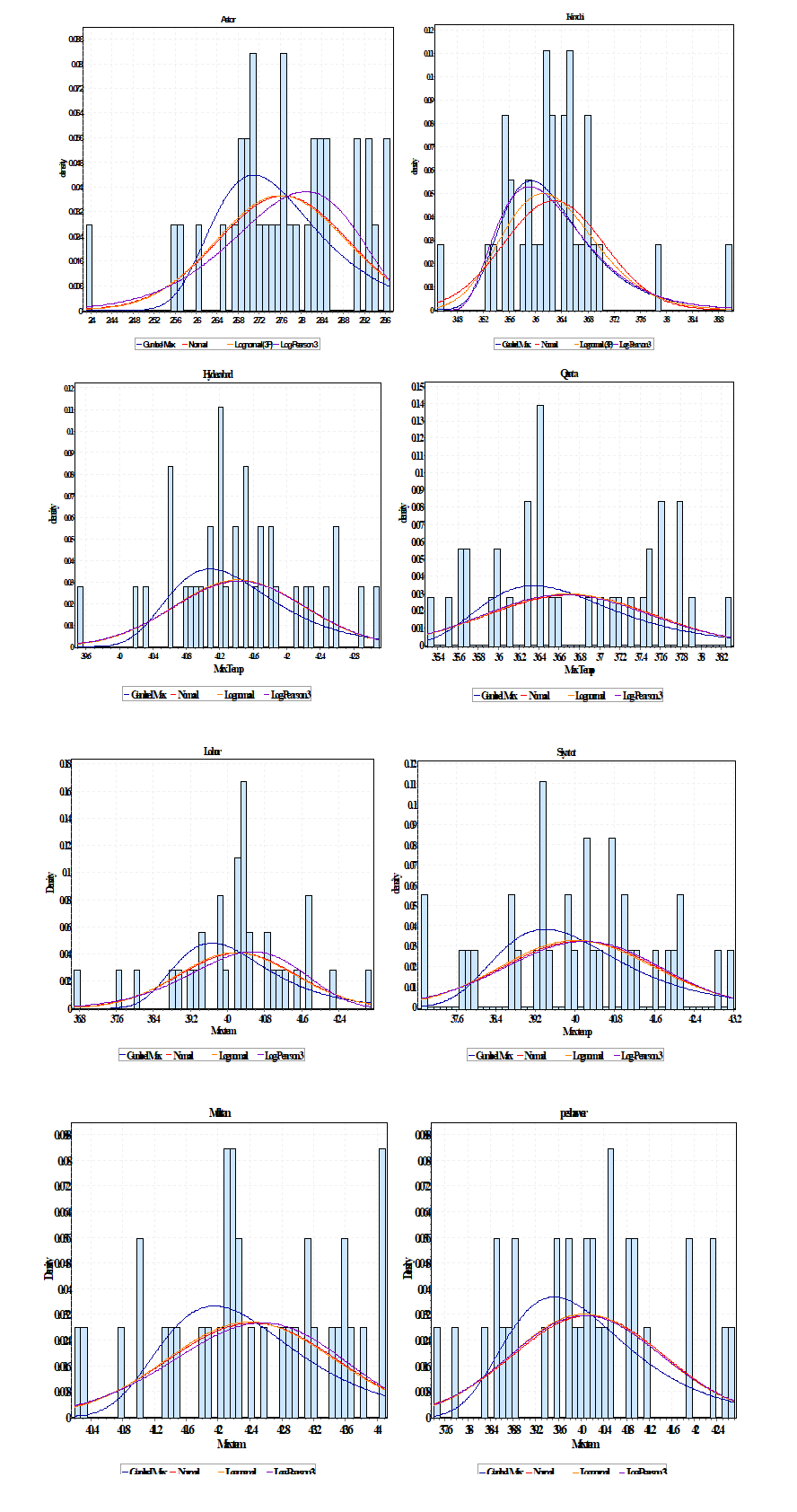
Fig. 3. PDF of annual maximum temperature (AMT) for eight stations
3.2 Probability distributions (PDs) selection
In order to model the extreme temperature, the selection of probability distributions for maximum temperature is important for measuring climate change in a region. Probability distributions, such as Generalized Normal (GNO), Generalize Logistics (GLO), Gumbel (GUM), Generalize Extreme value (GEV), Generalize Pareto (GPA), Logistic (LOG), Log Normal (LN), Normal, Log Pearson type3 and Pearson type3 (PE3) were considered in this study. Using goodness of fit tests, for example Kolmogorov Smirnov test, Anderson Darling test, and chi square test. The results of statistical data for most suitable distributions are recorded in Tables 4, 5, 6. Among all PDs select a best- fitted distribution for every station on the basis of smallest goodness of fit test. According to AD goodness of fit test, GEV is most suitable distribution for four stations, namely Quetta, Sialkot, Multan and Peshawar. However, GLO is the best-fitted distribution for Astor, Karachi, Hyderabad and Lahore; see Table 4 for more details. It was found that the KS fit test that GEV is best for Astore, Hyderabad, Quetta and Peshawar stations. The GLO is the most suitable distribution for Karachi, Lahore and Sialkot stations, while GPA is fit distribution for Multan as shown in Table 5.
L-skewness, L-coefficient of Variation (L-CV) and L-kurtosis of eight sites are presented in Table 3. It follows that Karachi and Lahore stations have higher L- kurtosis and skewness than the other sites. Quetta has the lowest L- kurtosis, but moderate L- CV and L – skewness. Astore, Hyderabad, Sialkot and Peshawar stations have moderate L-kurtosis. All stations have lower L-CV.
Table 3. Sample L-Ratios for different stations
|
Location |
L-CV |
L-SKEWNESS |
L-KURTOSIS |
|
Astore |
0.0253 |
-0.0613 |
0.1540 |
|
Karachi |
0.0199 |
0.1785 |
0.2743 |
|
Hyderabad |
0.0107 |
0.0319 |
0.1641 |
|
Quetta |
0.0129 |
0.0287 |
0.0040 |
|
Lahore |
0.0171 |
0.0654 |
0.2529 |
|
Sialkot |
0.0222 |
-0.0313 |
0.1318 |
|
Multan |
0.0144 |
-0.0509 |
0.0825 |
|
Peshawar |
0.0199 |
0.0140 |
0.1311 |
Table 4. Goodness of fit Anderson-Darling (AD) test
|
Location |
Goodness of fit AD test |
Best fitted distribution |
||
|
GEV |
GPA |
GLO |
||
|
Astor |
0.3212 |
8.1367 |
0.2829 |
GLO |
|
Karachi |
0.72908 |
8.5408 |
0.61973 |
GLO |
|
Hyderabad |
0.20012 |
7.9340 |
0.19206 |
GLO |
|
Quetta |
0.51756 |
4.1486 |
1.0526 |
GEV |
|
Lahore |
4.3107 |
8.5077 |
0.36335 |
GLO |
|
Sialkot |
0.14974 |
7.8522 |
0.19038 |
GEV |
|
Multan |
0.2408 |
11.1449 |
0.39611 |
GEV |
|
Peshawar |
0.32044 |
8.0336 |
0.3584 |
GEV |
Table 5. Goodness of fit Kolmogorov Simonov (KS) test
|
Location |
Goodness of fit KS test |
Best fitted distribution |
||
|
GEV |
GPA |
GLO |
||
|
Astor |
0.0823 |
0.1270 |
0.0851 |
GEV |
|
Karachi |
0.1286 |
0.1479 |
0.1210 |
GLO |
|
Hyderabad |
0.0707 |
0.1041 |
0.0783 |
GEV |
|
Quetta |
0.1317 |
0.8106 |
0.1670 |
GEV |
|
Lahore |
0.1331 |
0.1548 |
0.1296 |
GLO |
|
Sialkot |
0.0626 |
0.1086 |
0.0592 |
GLO |
|
Multan |
0.0934 |
0.0900 |
0.0908 |
GPA |
|
Peshawar |
0.0829 |
0.1115 |
0.7562 |
GEV |
Chi-square test was also used to find the most appropriate PDF for the eight stations. The primary result and the selected most suitable PDF are shown in Table 6. It follows from Table 6 that LP3 distribution is best fit for Hyderabad, Quetta, Lahore, Sialkot and Peshawar stations. However, normal and LN, respectively, are the most suitable distributions for Astore and Karachi, Lahore. Therefore, we conclude that the LP3 distribution may be the best-fitted PDF for predicting the annual maximum temperature.
Table 6. For best fit PDF using Chi-square test
|
Location |
chi square |
Best fit PDF |
|||
|
Normal |
LN |
LP3 |
Gumbel |
||
|
Astor |
0.549 |
0.56903 |
1.7771 |
1.4489 |
Normal |
|
Karachi |
5.7471 |
3.6249 |
4.6474 |
4.8279 |
LN |
|
Hyderabad |
0.9619 |
0.29377 |
0.2237 |
0.3509 |
LP3 |
|
Quetta |
8.9984 |
4.8151 |
4.4231 |
6.7743 |
LP3 |
|
Lahore |
1.0622 |
7.8225 |
1.3716 |
6.5793 |
LP3 |
|
Sialkot |
1.3608 |
1.9896 |
1.4231 |
2.5058 |
LP3 |
|
Multan |
1.2707 |
1.2978 |
2.2353 |
2.2985 |
LN |
|
Peshawar |
1.9627 |
4.8974 |
4.8731 |
6.7003 |
LP3 |
The KS goodness of fit test indicates that the GEV distribution is most appropriate for four stations, GPA is best-fitted for one station, and GLO is the best for the remaining three stations, however for the ADF test GEV and GPA are best fitted distributions for each four stations. In Chi-square test, LP3 is the best distribution for five stations, Normal distribution is the best for one and Log Normal distribution is good for the remaining two stations.
L-moments ratio diagram is appropriate tool to differentiate the distributions of the candidate descriptive data. The sample L kurtosis and L skewness as a scatter plot then compared to the hypothetical L moment ratio curve of the candidate distribution. Graphic field of vision L scale diagram shows one of the ten PDs as the picture shows, after evaluation each station separately see in Figure 4 and find PE3, NOR, LOG, EXP, GUM, and UNI distribution shown is inferior suitable than other PDs (GEV, GPA, GLO and GNO) in Figure 4 shows that the data series of high L kurtosis and L skewness followed GLO distribution. L kurtosis and lowest skewness of the data trend to follow GNO and GEV distribution.
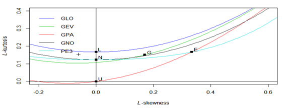
Fig. 4. L-ratio diagram for six probability distributions
For three stations (Karachi, Multan and Peshawar), Figure 5 indicates Q-Q plots fitting results matched the observed values. It is obvious from Fig 5(a) that GEV, GLO and GPA distributions perform well in expressing the extreme left and right tails, while the outcomes of GPA and GEV distribution is nearly unbiased the GLO distribution in QQ plot at Karachi station yields a low temperature than usually observed samples and the sequence of Karachi stations is much skewed. Also, the p-p plots in Fig5 (b) display the distributions of GEV, GPA and GLO. All the outcome of pp plots fit well the observed data. In other words, most of the observed points are close to a straight line GLO, GEV and GPA distributions.
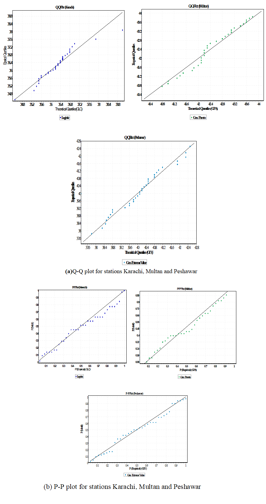
Fig. 5. Q-Q plots and P-P plots of best-fitted distributions.
The authors acknowledge funding from the National Natural Science Foundation of China (NSFC) (Grant No. 41875084).
Afzaal, M., Haroon, M. A., and Zaman, Q. 2009: Interdecadal oscillations and the warming trend in the area-weighted annual mean temperature of Pakistan. Pak. J. Meteorology, 6 (11), 13-19.
Alam, J., Muzzammil, M., and Khan, M. K. 2016: Regional flood frequency analysis: comparison of L-moment and conventional approaches for an Indian catchment. ISH J Hydraul Eng, 22(3), 247-253.
View ArticleBarnett, T. P., Adam, J. C., and Lettenmaier, D. P. 2005: Potential impacts of a warming climate on water availability in snow-dominated regions. Nature, 438(7066), 303. PMid:16292301
View Article PubMed/NCBIBozyurt, O., and Özdemir, M. A. 2014: The relations between north Atlantic oscillation and minimum temperature in Turkey. Procedia-Social and Behavioral Sciences, 120, 532-537.
View ArticleCui, L., Wang, L., Lai, Z., Tian, Q., Liu, W., and Li, J. 2017: Innovative trend analysis of annual and seasonal air temperature and rainfall in the Yangtze River Basin, China during 1960-2015. J ATMOS SOL-TERR PHY, 164, 48-59.
View ArticleDickey, D. A. 1976: Estimation and hypothesis testing in nonstationary time series.
Dickey, D. A., and Fuller, W. A. 1979: Distribution of the estimators for autoregressive time series with a unit root. Journal of the American statistical association, 74(366a), 427-431.
View ArticleFrías, M. D., Mínguez, R., Gutiérrez, J. M., and Méndez, F. J. 2012: Future regional projections of extreme temperatures in Europe: a nonstationary seasonal approach. Climatic Change, 113(2), 371-392.
View ArticleFuller, W. A. 1976: Introduction to Statistical Time Series, New York: JohnWiley. FullerIntroduction to Statistical Time Series1976.
Gilbert, R. O. 1987: Statistical methods for environmental pollution monitoring: John Wiley and Sons.
Hamed, K., and Rao, A. R. 1999: Flood frequency analysis: CRC press.
Hasan, H., Radi, N. A., and Kassim, S. 2012: Modeling of extreme temperature using generalized extreme value (GEV) distribution: A case study of Penang. Paper presented at the Proceedings of the world congress on engineering.
Hosking, J. R., and Wallis, J. R. 1987: Parameter and quantile estimation for the generalized Pareto distribution. Technometrics, 29(3), 339-349.
View ArticleHosking, J. R. M. 1990: L‐moments: Analysis and estimation of distributions using linear combinations of order statistics. J R STAT SOC B (Methodological), 52(1), 105-124.
View ArticleHosking, J. R. M., and Wallis, J. R. 2005: Regional frequency analysis: an approach based on L-moments: Cambridge University Press.
Huang, D., Yan, P., Xiao, X., Zhu, J., Tang, X., Huang, A., and Cheng, J. 2019: The tri-pole relation among daily mean temperature, atmospheric moisture and precipitation intensity over China. GLOBAL PLANET CHANGE, 179, 1-9.
View ArticleHuang, K., Chen, L., Zhou, J., Zhang, J., and Singh, V. P. 2018: Flood hydrograph coincidence analysis for mainstream and its tributaries. J HYDROL, 565, 341-353.
View ArticleKarpouzos, D., Kavalieratou, S., and Babajimopoulos, C. 2010: Trend analysis of precipitation data in Pieria Region (Greece). European Water, 30, 31-40.
Kendall, M. 1975: Rank Correlation Methods, Book Series, Charles Griffin: Oxford University Press, USA, London.
Kunz, M., Mohr, S., Rauthe, M., Lux, R., and Kottmeier, C. 2010: Assessment of extreme wind speeds from Regional Climate Models-Part 1: Estimation of return values and their evaluation. NHESS, 10(4), 907-922.
View ArticleLawan, S., Abidin, W., Chai, W., Baharun, A., and Masri, T. 2015: Statistical Modelling of Long-Term Wind Speed Data. AJCSIT, 3, 1-6.
View ArticleLi, Q., Dong, W., and Jones, P. 2019: Continental Scale Surface Air Temperature Variations: Experience Derived from the Chinese Region. Earth-Sci. Rev, 102998.
View ArticleMann, H. B. 1945: Nonparametric tests against trend. Econometrica: Journal of the Econometric Society, 245-259.
View ArticleMann, H. B., and Whitney, D. R. 1947: On a test of whether one of two random variables is stochastically larger than the other. The annals of mathematical statistics, 50-60.
View ArticleMasud, M. B., Soni, P., Shrestha, S., and Tripathi, N. K. 2016: Changes in climate extremes over North Thailand, 1960-2099. INT J CLIMATOL, 2016.
View ArticleNaghettini, M. 2017: Fundamentals of statistical hydrology: Springer.
View ArticleOzer, P., and Mahamoud, A. 2013: Recent extreme precipitation and temperature changes in Djibouti City (1966-2011). INT J CLIMATOL, 2013.
View ArticleRajabi, M., and Modarres, R. 2008: Extreme value frequency analysis of wind data from Isfahan, Iran. Journal of wind Engineering and industrial Aerodynamics, 96(1), 78-82.
View ArticleRasul, G., Dahe, Q., and Chaudhry, Q. 2008: Global warming and melting glaciers along southern slopes of HKH range. Pak. Jr. of Meteorology, 5(9).
Schmidt, G. A., Shindell, D. T., and Tsigaridis, K. 2014: Reconciling warming trends. Nature Geoscience, 7(3), 158.
View Article