Introduction
With the current rapid improvement in socioeconomic development, industrialization, and urbanization, urban water scarcity is becoming an overwhelmingly urgent issue on a global scale, and this is particularly prominent in China (Loomis et al., 2019). For example, the average annual water scarcity in China is up to 4.00 × 10⁸ m3, nearly two-thirds of China’s cities are suffering from a water shortage, and 443–525 million city people live with high water scarcity. Meanwhile, China’s urban water consumption continues to increase at an annual rate of 4–8% over the most recent decade (Wang et al., 2019). The conflict between increased water demand and limited available water resources has become particularly evident in most cities in China. Currently, urban water resource management patterns mainly focus on the reasonable exploitation and effective utilization of conventional water resources (including surface and underground water). In fact, nonconventional water resources, such as rainwater and reclaimed water, have significant advantages in regard to water resource allocation and management (Ye et al., 2018). For instance, the utilization of rainwater has the effect of reducing the water supply cost by replacing potable water used for flushing toilets and watering of gardens, and reclaimed water distributes for industrial demand with an overall positive environmental impact. The combination of conventional and nonconventional water resources from a quantity and quality viewpoint is thus expected.
In addition to water scarcity, modern urban water resource management is also confronted with the huge challenges presented by increasingly frequent urban flooding, which can cause substantial economic damage and human distress (Kundzewicz et al., 2018). Over the last decades, annual urban flooding damage in China has exceeded 10 billion USD, and the number of flood fatalities is greater than approximately 1,000 (Kundzewicz et al., 2019). Moreover, a series of research on the water resource management under climate change indicated that the climate change could aggravate water scarcity seriously and cause urban flooding frequently through affecting regional rainfall, temperature, evaporation, and hydrological cycle, leading to a huge challenge on water resource management (Shang et al., 2015; Mahmoud and Gan, 2018; Xia et al., 2019; Zhang et al., 2019). In order to deal with such challenges, the Chinese government initiated the “Sponge City” Program in 2013, which incorporates (LID) concepts to improve the urban drainage infrastructure and address urban flooding (Song et al., 2019; Xu et al., 2019). As a sustainable, innovative, and effective stormwater runoff control method, LID projects have advantages in controlling stormwater and urban runoff and storing rainwater as underground water resources compared with non-LID projects. However, the high construction cost associated with these projects may trigger excessive economic burden, which has a negative influence on the development and application of LID technologies. Moreover, many factors, including socioeconomic, meteorological, geographic, and environmental aspects, are involved in the selection and placement processes of LID projects, which bring significant difficulties to the formulation of the LID project optimization models and generation of effective solutions. Therefore, it is important to develop an effective method for optimizing LID project implementation schemes under complexities that improve water use efficiency, explore nonconventional water resources, and control urban flooding with a minimum cost.
For urban water resource management, considering system factors comprehensively, establishing LID projects rationally, combining nonconventional and conventional water resources effectively, dealing with the impact of climate change, and formulating water sources allocations optimization model are suitable methods for resolving urban water scarcity and flood control, and such approaches have been the focus of many studies in recent years (Mainuddin et al., 1997; Shangguan et al., 2002; Wang et al., 2008; Liu et al., 2011; Sample and Liu, 2014; Bekchanov et al., 2015; Palanisamy and Chui, 2015; Palla and Gnecco, 2015; Eckart et al., 2018; Xu et al., 2018; Ye et al., 2018; Helmia et al., 2019; Huang and Lee, 2019). For instance, Shangguan et al. (2002) developed a recurrence control model for regional optimal allocation of water resource for obtaining maximum efficiency. Liu et al. (2011) presented an optimization approach for the integrated management of water resources, including both nonconventional and conventional water resources. Xu et al. (2018) proposed an optimal water allocation model for industrial sectors based on water footprint accounting to optimize the allocation of nonconventional and conventional water resources in Dalian. Ye et al. (2018) presented a multi-objective optimization model to help optimize the allocation of water resources to different water users in Beijing. Sample and Liu (2014) developed a rainwater analysis and simulation model to optimize rainwater harvesting systems for water supply and runoff capture. Eckart et al. (2018) established a management model to optimize LID implementation strategies with the objective of minimizing peak flow. Huang and Lee (2019) proposed a programming model to solve water shortage of Taiwan under the impact of climate change. Helmi et al. (2019) developed a modeling tool to allocate LID projects in a cost-optimized method. However, above studies mainly sought to establish an optimization model for water resource allocation or LID projects, which considered only single objective for optimization, while in the real practice, there is more than one issue need to be taken into account simultaneously when designing and executing the water resource management strategies, for the sake of achieving a balance among them.
In fact with the increased complexity and our in-depth understanding in the urban water resource system, it is apparent that there is no absolute deterministic water allocation system. Specifically, the water demand exhibits a random nature that is subject to multiple variables, including meteorological factors, socioeconomic conditions, and deviations caused by the subjective judgments and understandings of humans. For example, the ecological water demand would be different with the change of runoff and biodiversity. Similarly, some economic and engineering factors, which are influenced by the resource availability, technical conditions, and policy regulations, fluctuate in the small ranges. For instance, the supply price of transfer water would fluctuate between 8.8 and 9.2 Yuan/m3 due to the impact of different technical conditions. Such uncertainties lead to significant difficulties in formulating urban water resource allocation models and generating an optimal management pattern. Currently, a large amount of uncertain optimization techniques have been developed by many researchers with the aim of solving urban water resource management problems (Huang, 1988; Liu et al., 2008; Qin and Huang, 2009; Qin et al., 2011; Dai et al., 2018; Xu et al., 2018; Zhang et al., 2019). For example, Dai et al. (2018) presented a Gini coefficient–based stochastic optimization model for supporting water resource allocation on a watershed scale. Xu et al. (2018) developed a stochastic-based water allocation optimization model on a watershed scale for supporting water supply planning and wetland restoration activities of the Xiaoqing River watershed. Zhang et al. (2019) proposed an interval multi-objective multi-stage stochastic programming model for finding a reasonable water storage scale and optimizing limited irrigation water resource. Based on the above studies, it can be concluded that many researchers have focused on dealing with the randomness inherent in urban water resource management. However, the above studies mainly utilized random variables with a known distribution type to describe the uncertainties involved in the water resource system, and they rarely observed that water demands in the real world may be subject to twofold randomness with incomplete or uncertain information. Specifically, it is first assumed that the water demands ξ are expressed as the random variables with the normal distributions, that is, ξ ∼ N (μ, δ2), where μ and δ denote the mean value and standard deviation, respectively. Based on various survey and estimation results from n group of respondents, n groups of random variables could be obtained, that is, (μ1, δ12), (μ2, δ22), (μn, δn2), such that μ and δ values are more suitable to be random variables (based on the collected data above) rather than fixed values as are traditional random variables (Xu et al., 2014). Hence, the parameters μ and σ should be described as new random variables, which are the so-called birandom variables, a concept first proposed by Peng and Liu (2007). This concept has been successfully applied to the flow shop scheduling problem, vendor selection problem, and hydropower station operation planning problem (Xu and Zhou, 2009; Xu and Ding, 2011; Xu and Tao, 2012).
As mentioned above, following three aspects of urban water resource management still need to be improved. First, current optimization models often pay attention to only one aspect of water resource allocation or LID project exploration. In fact, it is necessary to develop a comprehensive optimization model that incorporates the exploration of LID projects into the urban water management scheme. Second, because water demands directly affect the accuracy and rationality of the results due to the supply–demand constraint, it is important to develop a birandom optimization method to avoid the deviation caused by the birandomness of the water demands. Third, the climate change exerts the influences on the water availability and the occurrence of urban flood, which should be incorporated into the optimization model for integrated water resource management. As such, the main goal of this study was to develop a (MIBCCP) model under climate change for supporting the urban water resource management. The proposed model aims to optimize water resource allocation and address the urban flooding under uncertainties and different climate change scenarios, while minimizing the total system costs and maximizing the treated pollutant amount. The rest of this study is organized as follows: Materials and Methods introduce the descriptions of the compromise programming, birandom chance-constrained programming, and interval linear programming and describe formulation and the solution procedure of the MIBCCP model. An overview of the reference education park and the MIBCCP model for this park are proposed in Case Study. In Results Analysis and Discussion, the variations in the obtained solutions and impact of climate change on water resource management are analyzed and discussed. Finally, the conclusions summarizing this study are presented in the last section.
Methodology
To establish a cost-effective and environmentally friendly water resource management pattern, multiple objectives for the programming model should be taken under consideration, so that the model is capable of tackling the economic and environmental objectives simultaneously. Moreover, the estimation and expression of uncertain factors are critical for generating a rational and reliable management strategy of the urban water system, as many of the system parameters are associated with various types of the uncertainties. Therefore, an inexact multi-objective equilibrium chance-constrained programming model with the birandom and interval variables (i.e., MIBCCP) was developed for addressing these issues.
Preliminary Definitions and Descriptions of Proposed a Multi-Objective Interval Birandom Chance-Constrained Programming Model
In this section, some definitions, conceptions, and descriptions associated with compromise programming, birandom parameters, and interval numbers are described first in order to formulate and solve the proposed MIBCCP model.
Compromise Programming
Currently, many methods are available for solving multi-objective programming problems, among which the compromise programming is the most commonly used. The solution algorithm of compromise programming is based on the concept of a distance scale dp, a point which has the shortest distance to the ideal solution from the noninferior solution set. The total performance of all objective functions can be written as follows:
where
Introduction of Birandom Variable following the Normal Distribution
Birandom variable, a concept first proposed by Peng and Liu (2007), is a useful tool to deal with problems with twofold randomness and has been successfully applied to many fields (Xu and Zhou, 2009; Xu and Ding, 2011; Xu and Tao, 2012). In this study, the random variable following the normal distribution is considered as the example. For any ω, ξ(ω) is a birandom variable with normal distribution and is expressed as
Definition 2.1. A n-dimensional birandom vector ξ is a map from the probability space (Ω, A, Pr) to a collection of n-dimensional random vectors such that Pr{ξ(ω) ∈ B} is a measurable function with respect to ω for any Borel set B of the real space Rn. Especially, ξ is called a birandom variable as n = 1.
Example 2.1. A birandom variable ξ is assumed to follow the normal distribution, if for each ω, ξ(ω) is a random variable with normal distribution, denoted by N(μ(ω), σ2(ω)), where μ(ω), σ(ω) are the random variables defined on the probability space (Ω, A, Pr).
Lemma 2.1. Let ξ = (ξ1, ξ2, …, ξn) be a birandom vector and f be a Borel measurable function from Rn to R. Then f(ξ) is a birandom variable.Let ξ1 and ξ2 be two birandom variables defined on the probability spaces (Ω1, A1, Pr1) and (Ω2, A2, Pr2), respectively. Then ξ = ξ1 + ξ2 is a birandom variable on (Ω1 × Ω2, A1 × A2, Pr1 × Pr2) defined by ξ (ω1, ω2) = ξ1 (ω1) + ξ2 (ω2), (ω1, ω2) ∈ (Ω1 × Ω2).
Interval Number
The interval number is composed of the lower bound and upper bound, which is depicted in Eq. 1, where the items
Let
Multi-Objective Interval Birandom Chance-Constrained Programming
As stated in the Introduction section, the uncertainties associated with the urban water resource management system not only exhibit the random characteristics but also fluctuate in the small ranges. Therefore, in this study, an integrated uncertain multi-objective optimization model including the birandom parameters and interval numbers (MIBCCP) is developed for tackling two types of uncertainties.
Subject to:
where two objective functions
The first and critical step of solving model 3 is to combine two objective functions into one objective through designing various weight coefficients (i.e., w1 and w2).
where
Next, the constraint with birandom variables (3c) is converted into its interval equivalent based on the birandom equilibrium chance-constrained algorithm. The selection of the equilibrium chance measure is because it is a real number and is convenient for decision-makers to rank potential solutions (Peng and Liu, 2007). The original stochastic constraint could be reformulated as follows:
where αr represent predetermined probability violation levels. The principle of designing αr value is ensuring its ranges are wide enough. In order to generate a variety of decision alternatives and provide more choosing opportunities to decision-makers, a relatively wide range of designed parameter is necessary. Referring to the studies (Xu et al., 2009; Wang et al., 2018), in this study, the constraint violation level is designed as 0.01, 0.05, and 0.1, respectively.
Then, the interactive two-step algorithm proposed by Huang et al. (1992) is used for transforming the intermediate interval linear programming model into two submodels, which correspond to the upper and lower bounds of objective function values, respectively. The submodel corresponding to the lower bound of objective function is formulated first as (Xu and Zhou, 2009; Xu and Tao, 2012):
Subject to:
Based on obtained solutions from model 6, the submodel representing the upper bound of the objective function
Subject to:
Finally, the solutions of objective values and decision variables under various αr values are obtained, that is,
Step 1: Investigate the water resource management system and recognize system structure and components, respectively.
Step 2: Identify all types of uncertain variables as the birandom variables and interval numbers and determine the objective function and constraints in the optimization model.
Step 3: Establish an MIBCCP model based on step 1 and step 2.
Step 4: Combine two objectives into a single objective based on the compromise programming method.
Step 5: Convert the birandom constraints into their respective interval equivalents based on equilibrium chance-constrained measure.
Step 6: Transform the interval model into two submodels through an interactive two-step algorithm, which correspond to the lower bound and upper bound models, respectively.
Step 7: Solve two submodels and generate the final solutions of objective values and decision variables under various conditions.
FIGURE 1
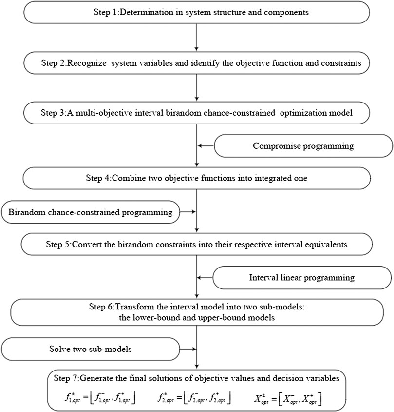
FIGURE 1. Main procedure of formulating and solving a multi-objective interval birandom chance-constrained programming model.
Case Study
Overview of the Study Area
To demonstrate the advancement of the proposed optimization model for optimizing the allocation of water resource and addressing urban flooding with minimal LID project construction cost, an education park water system in Tianjin, China, was taken as an example. As shown in Figure 2, the reference park is a national demonstration zone of vocational education reform and innovation in China, located at latitude 38°34′−40°15′N and longitude 116°43′−118°4′E, and it covers an area of 37 km2 with a total population of 0.2 million. The annual rainfall is about 480 –520 mm, 75% of which is concentrated in the months of June, July, and August. As a demonstration area constructed with “three-zone linkage” (educational zone, residential zone, and industrial zone), the reference park clearly has high requirements in regard to water availability and water supply safety. However, its existing water provision is incapable of meeting the scale expansion needs of the park in the future, which is mainly reflected in the following aspects: i) water scarcity is an urgent problem in this area. The water resource per capita is 160 m3/a, which is only about 7% of the average level in China; ii) the major water source for this park is the local reservoir, and no alternative sources are available. As such, this single water source will affect the water supply security; iii) the capability of water conservation and retention has declined due to the decrease in puddle and lake areas; moreover, increased concrete areas has also reduced the penetration of rainwater into the soil. The on-site survey result indicated that this park often undergoes flooding, which would be exacerbated under climate change; iv) intrinsic uncertainties are associated with the water resource system of this park, including the volatility in water demands and fluctuations in the prices of water resource. The current water resource management plan neglects the uncertain features and potential risk caused by climate change that can affect the accuracy and rationality of the water allocation strategy. Therefore, it is important that an effective water resource optimization model is formulated to help mitigate and/or solve the above issues.
FIGURE 2
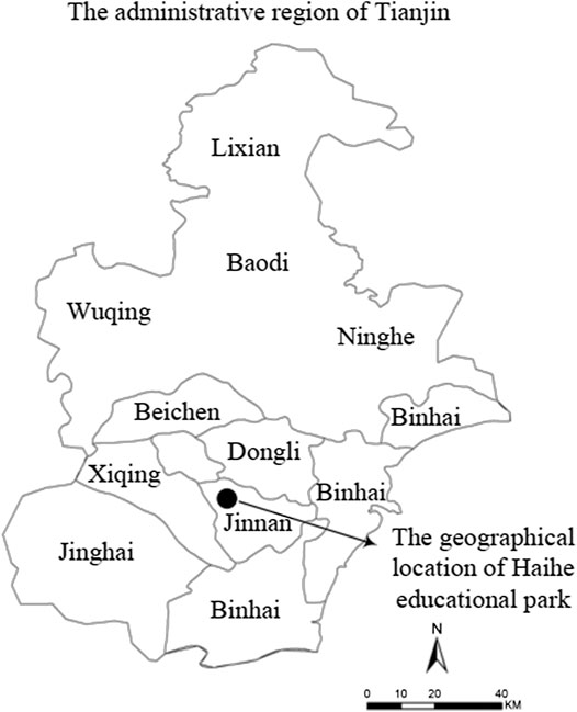
FIGURE 2. Demonstration of study area.
Impact of Climate Change on the Study Area
Over the last decades, climate change has significantly aggravated water scarcity and intensified frequency of extreme weather events (such as urban flooding and droughts) in China (Niu et al., 2008; Yu et al., 2008; Guo et al., 2019). Hence, it is necessary to detect future changes in rainfall over a region by using the simulation techniques in order to identify the influence exerted by climate change and generate an optimal water resource management strategy. PRECIS is a regional climate model system developed at the Met Office Hadley Centre, United Kingdom (Rao et al., 2014). It is advantageous in simulating the change trend of climatic variables due to its easy-to-use operation, high computational precision, and wide suitability. In this study, the average annual rainfall in the reference park was predicted under four periods (2025, 2050, 2075, and 2100) and two emission scenarios (RCP4.5 and RCP8.5) by the PRECIS model, which are shown in Table 1. From Table 1, it can be seen that the average annual rainfall shows an upward trend among four periods under the impact of climate change in the future.
TABLE 1
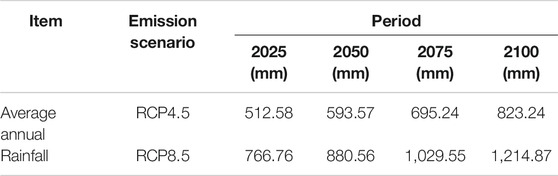
TABLE 1. Average annual rainfall under various periods and scenarios.
Description of the Water Resource System
Figure 3 presents the water network in the studied region. Based on the natural conditions, geographical position, and surface runoff of the reference park, the water resource management system for this park is conceptualized as 12 nodes, including four water sources, six water users, and LID, and non-LID projects. The major water sources are transfer water, tap water, reclaimed water, and rain water, which are used for living, industry, tertiary industry, construction, ecology, and other water users. Considering a water-saving plan, green ecological requirements, and traditional water source allocation principles of the city of Tianjin, this study made some adjustment as follows: i) “planning of recycled water utilization of Tianjin” highlights that the utilization of reclaimed water should be considered for livelihood water with the maximal value of 30 L/d per capita. Hence, the water sources for livelihood water would be transfer water, tap water, and reclaimed water. ii) According to “technical specifications for construction and community rainwater utilization engineering,” rainwater can be used for green space irrigation and road watering. Therefore, the demand for ecology water could be met by reclaimed water and rainwater, which are harvested via the LID and non-LID projects in this study. iii) Other water users should include the water source loss caused by water transfer, including transfer water loss and tap water loss.
FIGURE 3
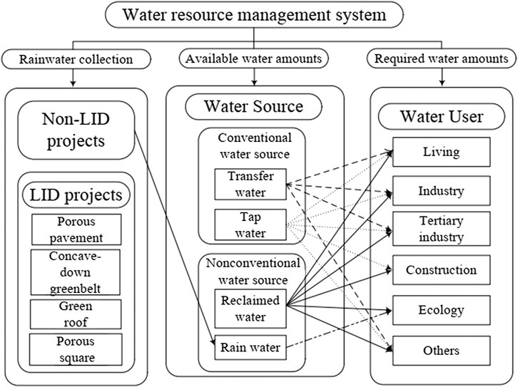
FIGURE 3. Regional water supply system.
Formulation of the Multi-Objective Interval Birandom Chance-Constrained Programming Model Under Climate Change
As mentioned in the above sections, the generation and execution of a rational water resource management strategy under climate change, including the determination of the system components, design of the system operation pattern, and generation of water allocation alternatives, are directly related to the coordinated development of local socioeconomy and environmental factors.
Therefore, the MIBCCP model for tackling the water supply problem of the park was formulated, as shown in Figure 4. This model was used to identify and determine the optimal water allocation strategy under climate change, which could enhance the economic efficiency, reduce environmental water pollution, and avoid the negative effects caused by various uncertainties associated with the water resource management system. The formulation and solution procedures of the MIBCCP model in this study are summarized as follows:
Step 1: Investigate the water resource management system and recognize system structure and confirm the impact of climate change.
Step 2: Identify all types of uncertain variables as the birandom variables and interval numbers and determine the objective function and constraints in the MIBCCP model based on step 1.
Step 3: Establish the MIBCCP model depended on step 2.
Step 4: Solve the MIBCCP model and generate the solutions of objective values and decision variables under different conditions.
Step 5: Analyze and discuss the results obtained in step 4 and support managers to make a trade-off between the economic benefits and environmental benefits, identify the relation between the system cost and the joint constraint violation risk, and deal with the impact of climate change.
FIGURE 4
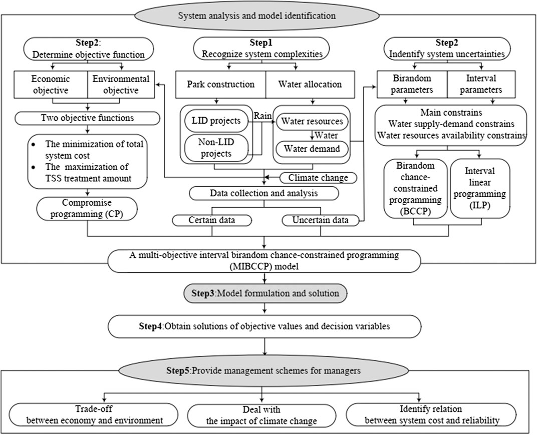
FIGURE 4. Water supply management diagram for the educational park in Tianjin.
Objective Functions
i. Economic objective
where
i. Environmental objective
where
Constraints
i. Constraint for water resource availability
(8c)
(8d)
(8e)
(8f)
where
ii. Constraint for the water supply–demand balance
(8g)
(8h)
(8i)
(8j)
(8k)
(8l)
where
iii. Constraint of conventional water resource utilization
(8m)
(8n)
(8o)
where GDP = gross domestic product of the reference park (104 RMB);
iv. Constraint of reclaimed water reuse rate
(8p)
where
v. Constraint of the LID projects
(8q)
(8r)
(8s)
(8t)
(8u)
(8v)
where Ap = available area of the pavement in the lark, m2; AG = available area of the greenbelt in the lark, m2; Ap = available area of the roof in the lark, m2; Ap = available area of the square in the lark, m2; Qys = rainfall runoff of the lark, m3; Fn,m = runoff coefficient of projects n at the construction area m; Qyh = average rainfall of the lark during one year, m3; Qyx = storage volume of rainfall, m. The constraints (8q) to (8t) are used to control the construction area of the LID projects in the pavement, greenbelt, roof, and square areas. The constraints (8u) to (8v) regulate the rainfall runoff and the rainwater availability, respectively.
vi. Other constraints
where θTs = transmission loss coefficient of transfer water; θTa = transmission loss coefficient of tap water. The constraints (8w) to (8x) regulate the transmission losses of the transfer water and tap water, respectively. The constraints (8y) to (8z) require the decision variables to be greater or equal to zero. Based on compromise programming and stochastic equilibrium chance-constrained programming methods described in Materials and Methods, two objectives (including economic and environmental objectives) were first combined into a single objective; then, the birandom constraints (including water supply–demand balance constraints) were converted into their interval equivalents; next, the interval form objective function and constraints were transferred to their respective two deterministic forms. Finally, the interval solutions under various constraints violation levels (i.e., 0.01, 0.05, and 0.1) were obtained, that is,
Data Information
The model parameters can be divided into two types in this study, which included engineering parameters and water resource system parameters.
Engineering Parameters
Engineering parameters composed of construction costs, runoff coefficients, TSS treatment efficiencies, and available areas of LID and non-LID projects, which are shown in Table 2. The available areas are subjected to the park-scale limitation and remain unchanged, where they are expressed as deterministic values that came from Tianjin Statistics Bureau. The construction cost and TSS treatment efficiency have significant variations caused by policy regulations and technical condition, where they exhibited the uncertain characteristics with known upper and lower bounds. Accordingly, it is essential to define them as the interval numbers.
TABLE 2
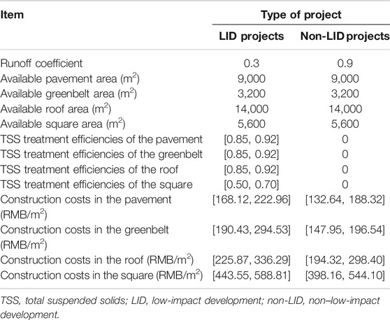
TABLE 2. Parameters associated with the low-impact development and non–low-impact development projects.
Water Resource System Parameters
According to on-site survey results, historical data record (from 2010 to 2018), Tianjin Statistics Bureau, and Tianjin Statistics yearbook, water resource system parameters include water provision cost, available water amount, and users’ requirements, and their detailed data information is displayed in Table 3. Among them, users’ requirements are affected by population, production scale, and local meteorological condition. Therefore, they are designed as the birandom variables with normal probability distribution. The water supply cost and available water amount own the small variation range and thus are assumed to be the interval number.
TABLE 3
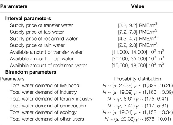
TABLE 3. Parameters related to the water resource system.
Results Analysis and Discussion
Results Analysis
Table 4 displays the optimal solutions of the MIBCCP model under different constraint violation levels (i.e., α) and different weight combinations. Based on the description of the interval linear programming in the Methodology section, the solutions for the two objective function values and some decision variables could be presented as interval numbers. For instance, when α = 0.1, w1 = 0.1, and w2 = 0.9, the TSS treatment amounts would range from 31.6 × 10³ to 34.2 × 10³ tons. The system costs would change from 35.75 to 43.77 million RMB. The transfer water amount allocated to livelihood would fluctuate from 6.07 to 8.47 million m3. The solutions of the two objectives correspond to the upper bound of the environmental benefit and the lower bound of the system costs, which are obtained under the most optimistic conditions (e.g., high TSS treatment efficiency as well as low construction and water allocation prices) when the interval decision variables (e.g., water resource allocation amounts) are at their lower bounds; although the solutions corresponding to the lower bound of the environmental benefit and the higher bound of the system costs are associated with the most conservative conditions when the water resource allocation amounts reach their higher bound levels. In fact, the flexibility and adjustability of the interval decision variables are beneficial for the decision-maker when inserting more implicit knowledge (e.g., socioeconomic conditions) into the optimize model so that they can formulate a more satisfactory and applicable decision scheme. Moreover, some interval decision variables indicate that there is no difference between their upper bound value and lower bound value. For example, when α = 0.1, w1 = 0.1, and w2 = 0.9, the solutions of 8.00 million m3 and 1.44 million m3 are the tap water amounts allocated to industry and tertiary industry users. This is because these decision variables are insensitive to the variations in interval parameters.
TABLE 4
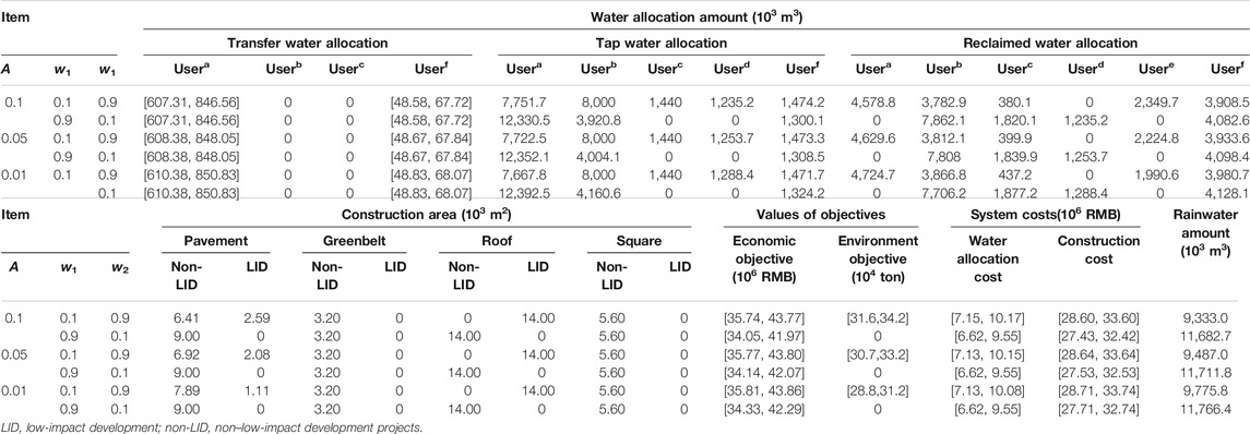
TABLE 4. Part of solutions of multi-objective interval birandom chance-constrained programming model under various α values and weight combinations.
Considering that the obtained solutions are affected by the interactive influence of the above two factors (weight coefficient combination and violation level), for the sake of reflecting the impact exerted by each factor, the variation trend of the solutions was analyzed under the context of changes to one factor as the other factor remains unchanged. First, when the three violation levels were maintained as stable (α = 0.1), the selection of the construction schemes exhibited an obvious difference under various weight combinations. The high w1 value would help to raise the economic benefits; otherwise, as w2 climbs, the environmental benefits would increase. For instance, the non-LID projects are favored when the system costs are more of a concern, where w1 = 0.9 and w2 = 0.1. Under α value of 0.1, the difference in values between the non-LID project construction area and LID project construction area for pavement, greenbelt, roof, and square areas were 9.0 × 10³, 3.2 × 10³, 14.0 × 10³, and 5.6 × 10³ m2, respectively. Conversely, with the change in weight combinations from w1 = 0.9 and w2 = 0.1 to w1 = 0.1 and w2 = 0.9, the difference in values would be 3.8×10³, 3.2×10³, −14.0×10³, and 5.6 × 10³ m2, respectively. This variation is because LID projects can bring increased environmental benefits. Moreover, selection of the water allocation strategy is also dependent on the weight coefficients. For example, it is established that the water demand of the tertiary industry is satisfied by tap water and reclaimed water with the values of 144 and 38.01 million m3, where w1 = 0.1 and w2 = 0.9. However, when the system focuses on the economic benefit (w1 = 0.9 and w2 = 0.1), reclaimed water with its low allocation price would be the preferred source, and thus, the water demand of the tertiary industry would be provided in total by reclaimed water. A similar situation was also reflected in the different climate change scenario and time period. For example, under the RPC 4.5 scenario, when w1 = 0.1 and w2 = 0.9, tap water would be used to meet the water demand of the construction industry in 2025, with the values of 123.5 million m3. When w1 = 0.9 and w2 = 0.1, the water demand of the tertiary industry would be provided in total by reclaimed water due to its high economic characteristic. The function of weight coefficients was to provide different water resource management schemes for managers. If the environmental quality is relatively poor and needs to be improved, managers should focus on the environmental benefits and choose the scheme under the high w2. Conversely, they could prefer to increase the economic benefits and select the scheme under the high w1.
Moreover, the variable situations of the obtained solutions under the different fixed weight coefficient combinations are discussed in order to examine the influences caused by violation level design on the generated decision schemes. First, when two weight coefficients are maintained as stable (w1 = 0.9 and w2 = 0.1), as the increase in the probabilistic level, the total water amounts supplied to four water users were decreased. For example, at the three α levels of 0.01, 0.05, and 0.1, the water amounts transferred to meet the demands of livelihood were 18,496.3, 18,435.9, and 18,403.6 × 103 m3, respectively; similarly, the water amounts allocated to industry and the rainwater amount collected by LID and non-LID projects increased from 9,333.0 and 11,866.8 × 103 m3 to 9,775.8 and 11,782.9 × 103 m3, respectively. Meanwhile, the results own the same trends under climate change. For example, under the RPC 8.5 scenario, when α increases from 0.01 to 0.1, the water demand of the construction industry provided by reclaimed water was reduced in 2,100, being from 1,288.4 × 103 to 1,235.2 × 103 m3; the tap water allocated to industry would decrease to 3,920.8 × 103 from 4,160.6 × 103 m3. The main reason for this result is that the decrease in α value meant the constraints with the birandom variables would be strict, such that the water demand amounts would increase. On the contrary, the increase in the violation level of α means that the satisfied extent of the constraint has become weak, leading to a decrease in the water demand.
The changes in the combinations of weight coefficients and violation levels exerted an influence on the decision variables, but they also influenced the objective value. The economic and environmental objectives under various weight combinations and violation levels were estimated and are shown in Figure 5A. From Figure 5A, it was apparent that regardless of the α levels, the values of two objectives both keep the same trend with the change in weight combinations, considering the obtained solutions are affected by the interactive influence of the above two factors (w and α); thus, in order to reflect the impact exerted by w, the variation trend of the solutions was analyzed under a stable constraint violation, which was selected as 0.1. Specifically, when w1 increased from 0.1 to 0.8 and w2 simultaneously decreased from 0.9 to 0.2 under α = 0.1, the economic objective and environmental objective remained unchanged with the values of 35.75, 43.77 million RMB and 31.6, 34.2 ×10³ tons. When w1 and w2 changed to 0.9 and 0.1, the two objectives decreased especially fast to 34.05, 41.97 million RMB and 0 tons. This indicated that the values of two objectives were insensitive to the weight shift before w1 reaches 0.8. Only when w1 = 0.9 and w2 = 0.1 could the solution of environmental objective would decrease, which means the decision-makers considering environmental benefits are not the key factor for determining the optimal water resource allocation strategy. Meanwhile, the solution of economic objective corresponding to the total cost of the system would decrease, which represents the decision-makers focus on the economic benefit and aim to reduce the system costs.
FIGURE 5
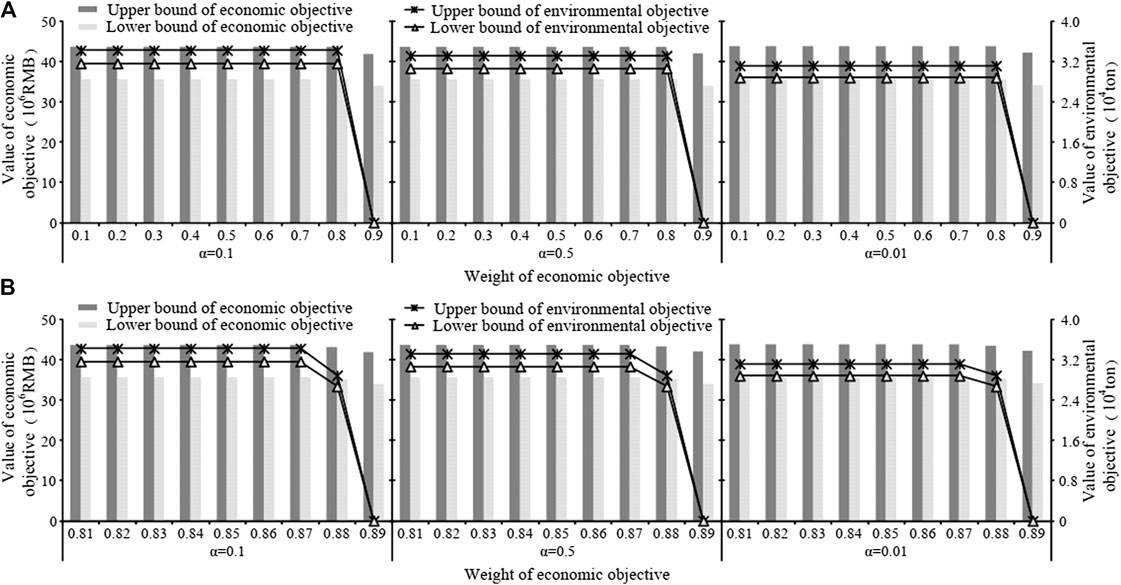
FIGURE 5. Economic and environmental objective values under various α values and weight combinations. (A) Weight of economic objective is from 0.1 to 0.9; (B) Weight of economic objective is from 0.81 to 0.89.
In order to further reflect the sensitive range of objective functions, two objectives values under different weight coefficients (changing between from w1 = 0.8, w2 = 0.2 and, w1 = 0.9, w2 = 0.1) were estimated and displayed in Figure 5B. As demonstrated in Figure 5B, it was apparent that the values of two objectives decreased fast only when w1 shifted from 0.87 to 0.89 and w2 ranged from 0.11 to 0.13, respectively. For example, under an α value of 0.1, TSS treatment amounts are 31.6, 34.2 ×10³ tons, 26.7, 28.9 ×10³ tons, and 0 ton under the three weight coefficient combinations (i.e., w1 = 0.87 and w2 = 0.13, w1 = 0.88 and w2 = 0.12, and w1 = 0.89 and w2 = 0.11). The total system costs also showed the similarly downward trend with the values of 35.75, 43.77, 35.27, 43.29, and 34.05, 41.97 million RMB. Hence, if the managers wanted other results for system costs and treatment amount of TSS, they could adjust the parameters of the optimization model by choosing different w1 and w2 values between the above range.
Apart from the weight coefficient combinations, the values of two objectives were also influenced by the levels of α. As shown in Figure 5A, various α values resulted in different solutions. The value of economic objective decreased with the increase in α value. In contrast, the value of environmental objective increased with the growth level of α. For example, when w1 = 0.1 and α increased from 0.01 to 0.1, the total treatment of TSS exhibited an upward trend from 28.8, 31.2 ×10³ tons to 31.6, 34.2 ×10³ tons. Inversely, the costs of the system decreased to 35.75, 43.77 million RMB from 35.71, 43.85 million RMB. This is because the α level represents the constraint violation risk of water supply–demand balance. The low α level corresponded to a low violation risk with a high water demand, leading to a high water allocation amount, which caused an increase in the system cost. Conversely, a high α value was associated with a high violation risk, which was accompanied by a low water supply amount. The variation in the α level provides a variety of water resource management schemes to the managers, which reflected the trade-off between the system economy and risk. Generally, the water demand can be divided into two categories: rigid demand and flexible demand. For example, the industrial water demand must be satisfied in its entirety subjected to its production characteristic. Conversely, the living water demand has a high elasticity and is able to reduce the water requirement through a series of water-saving measures under the water shortage scenario. The elastic characteristics of water demand allow the managers to design the water provision schemes according to local situation. Specifically, for the area where the economic development is relatively backward and simultaneously suffers from water shortage, it is suitable to select the scheme under the high α level which is capable of increasing the economic benefits and decreasing the water provision amounts, although it also may result in the high system failure risk. Conversely, the managers could choose the strategy under the low α level so that the water supply security would be enhanced by raising water supply amounts and system costs. Tianjin, as one of the most prosperous cities in China, always faces severe water shortage and thus has the superiority on economic development and the inferiority on water resource availability at the same time. Therefore, it is suggested that a compromise alternative (i.e., α = 0.95) be adopted as the decision basis for the generation of final water resource management scheme in this study, which is helpful in realizing the balance between system economy and failure risk.
Discussion
In order to evaluate the influence caused by climate change on the water resource management, the generated runoff of the studied region and LID project implementation scheme were estimated under the two climate change scenarios (RCP4.5 and RCP8.5) with four periods (2025, 2050, 2075, and 2100), which were displayed in Figure 6. As shown in Figure 6, under fixed α level, the runoff of the park and area of LID projects would increase from 2025 to 2100 under both two scenarios. For example, with an α value of 0.1, when the period changes from 2025 to 2100, the runoffs in the RCP4.5 and RCP8.5 scenarios would increase from 696.7 to 1,510.0 million m3 to 1,610.26 and 2,704.3 million m3; meanwhile, the areas of LID projects would be upward from 17.35 and 27.4 thousand m2 to 28.8 and 31.8 thousand m2, respectively. That is because the climate change could lead to the growths in regional rainwater and runoff, which might trigger the rainfall flood. The similar results were also reported by other studies (Zahmatkesh et al., 2014; Yoon et al., 2015; Guo et al. (2019a)). For instance, Zahmatkesh et al. (2014) found that climate change led to the increase in the urban stormwater runoff volume of the Bronx River watershed, New York City. Yoon et al. (2015) proposed a methodology for the evaluation of the overflow probability of urban streams under climate change in the Uicheon Basin of Korea and obtained results showed that 100-year peak flow in the future would increase by 58.1% compared with historical conditions. Moreover, to deal with the increase in the flooding risk caused by climate change, the LID project is recommended as climate mitigation measures in this research, which was capable of alleviating the adverse impact of increased stormwater based on the collection and retention facilities of the rainwater. The obtained results are consistent with the related studies, such as Guo et al. (2019b), Morvarid et al. (2019), and Hou et al. (2019). Specifically, it is concluded that the LID projects are beneficial to reduce the flooding risk and cope with the stormwater management issue arising from heavy rainfall under climate change. On the other hand, the above studies formulated the urban water management model with the aid of hydrological software (i.e., SWMM), which has excellent performance in describing the hydraulic connections and relationships among various water sources and users. In this study, an MIBCCP model based on compromise programming, birandom chance-constrained programming and interval linear programming is proposed for identifying the uncertainties associated with the urban water resource management system and generating a variety of water allocation patterns reflecting the trade-off between system economy and reliability; however, it also has difficulties in obtaining more accurate solutions due to oversimplified hydrologic and hydraulic equations. Therefore, it is necessary to enhance the accuracy and applicability of the proposed model through incorporating the output of some hydrological models into the optimization process.
FIGURE 6
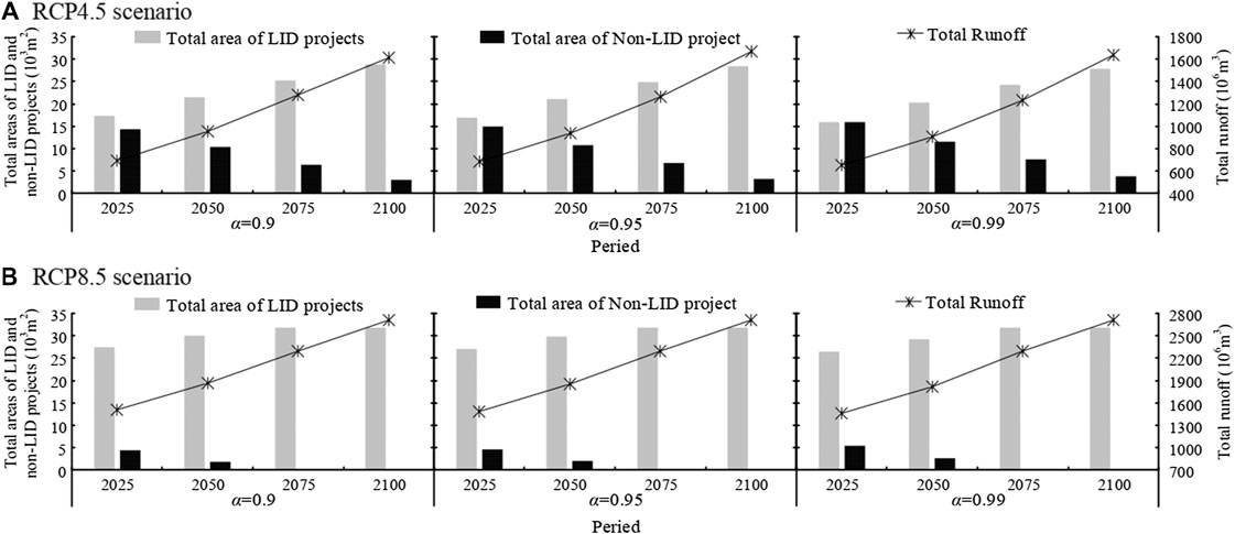
FIGURE 6. Variations in the runoff and low-impact development projects areas under two climate change scenarios. (A) RCP 4.5 scenario; (B) RCP 8.5 scenario.
Moreover, the MIBCCP model still needs to be improved, especially in the following three aspects. First, the objective function in this study is assumed as a linear form; in fact, system cost could exhibit the economy-of-scale feature, and the relationship between water supply cost and distance may be nonlinear, rather than the linear one. This will lead to a nonlinear objective function. Because the focus of this research is to apply birandom variables and interval numbers for supporting water resource management issue, it is thus desired to examine the possibility of the integrated model of MIBCCP and nonlinear programming in the future. Second, the compromise programming is used to combine two objectives into an integrated one. In fact, many types of multi-objective methods are available, such as the genetic algorithm and the interactive approximation algorithm. How to select an appropriate solution method through the comparison analysis is very critical. Third, two traditional objectives are considered in the MIBCCP model. In fact, other objectives, including the ecological stability and social acceptance, also obtained more attentions and thus deserved further research.
Conclusion
Under the urgency of rational water resource allocation and effective urban flooding control, a (MIBCCP) model under climate change is developed in this study. The MIBCCP model incorporates compromise programming, birandom chance-constrained programming, and interval linear programming within a general framework, where each technique offers a unique contribution toward the enhancement of the model capability in tackling the complexities and uncertainties. A water supply management system of educational park in Tianjin was used to demonstrate the applicability of the proposed method. A variety of water allocation patterns are obtained through adjusting predetermined constraint violation levels and weight combinations, which indicated that MIBCCP was useful in helping local managers gain in-depth insights into the water management system under climate change, realize the utilization of nonconventional water source and application in LID projects, and analyze the trade-offs between system economy and reliability, as well as establish the cost-effective environmentally friendly water provision strategies. Meanwhile, optimal construction schemes for LID projects under two scenarios were identified by the MIBCCP model to deal with the rainfall flood control issue under climate change. The successful application in the park is expectable for providing a good demonstration to the water management problem in other regions of China. In the future, high-precision hydrological simulation models and other multi-objective programming methods should be incorporated into the proposed model for tackling more complex issues.
Data Availability Statement
All datasets generated for this study are included in the article.
Author Contributions
YX, ZB, and GH conceived and designed the research. WL, HY, and ZB collected the data. YX, ZB, GH, and HY formulated the optimization model. ZB, YX, and GH performed the data analyses and manuscript preparation. ZB, YX, WL, and HY wrote the paper. GH, WL, and YX gave the comments and helped in revising the paper.
Funding
This research was supported by Joint Fund of State key Lab of Hydroscience and Institute of Internet of Waters Tsinghua-Ningxia Yinchuan [sklhse-2020-Iow10] and National Key Research and Development Plan (2018YFE0196000).
Conflict of Interest
The authors declare that the research was conducted in the absence of any commercial or financial relationships that could be construed as a potential conflict of interest.
References
Bajracharya, A. R., Bajracharya, S. R., Shrestha, A. B., and BikashMaharjan, S. (2018). Climate change impact assessment on the hydrological regime of the Kaligandaki Basin, Nepal. Sci. Total Environ. 625, 837–848. doi:10.1016/j.scitotenv.2017.12.332
Bekchanov, M., Bhaduri, A., and Ringler, C. (2015). Potential gains from water rights trading in the Aral Sea Basin. Agric. Water Manag. 152, 41–56. doi:10.1016/j.agwat.2014.12.011
Dai, C., Qin, X. S., Chen, Y., and Guo, H. C. (2018). Dealing with equality and benefit for water allocation in a lake watershed: a Gini-coefficient based stochastic optimization approach. J. Hydrol. 561, 322–334. doi:10.1016/j.jhydrol.2018.04.012
Eckart, K., McPhee, Z., and Bolisetti, T. (2018). Multiobjective optimization of low impact development stormwater controls. J. Hydrol. 562, 564–576. doi:10.1016/j.jhydrol.2018.04.068
Guo, J. H., Huang, G. H., Wang, X. Q., Li, Y. P., and Yang, L. (2018). Future changes in precipitation extremes over China projected by a regional climate model ensemble. Atmos. Environ. 188, 142–156. doi:10.1002/2016EF000433
Guo, L. M., Shan, N., Zhang, Y. G., Sun, F. B., Liu, W. B., Shi, Z. J., et al. (2019a). Separating the effects of climate change and human activity on water use efficiency over the Beijing-Tianjin Sand Source Region of China. Sci. Total Environ. 690, 584–595. doi:10.1016/j.scitotenv.2019.07.067
Guo, X. C., Du, P. F., Zhao, D. Q., and Li, M. (2019b). Modelling low impact development in watersheds using the storm water management model. Urban Water J. 16 (2), 146–155. doi:10.1080/1573062X.2019.1637440
Helmia, N. R., Verbeirena, B., Mijicb, A., Griensvena, A., and Bauwensa, W. (2019). Developing a modeling tool to allocate low impact development practices in a cost-optimized method. J. Hydrol. 573, 98–108. doi:10.1016/j.jhydrol.2019.03.017
Hou, J. M., Han, H., Qi, W. C., Guo, K. H., Li, Z. B., and Reinhard, H. (2019). Experimental investigation for impacts of rain storms and terrain slopes on low impact development effect in an idealized urban catchment. J. Hydrol. 579, 124176. doi:10.1016/j.jhydrol.2019.124176
Huang, G. H. (1988). A hybrid inexact-stochastic water management model. Eur. J. Oper. Res. 107 (1), 137–158. doi:10.1016/S0377-2217(97)00144-6
Huang, G. H., Baetz, B. W., and Patry, G. G. (1992). A grey linear programming approach for municipal solid waste management planning under uncertainty. Civil Eng. Syst. 9, 319–335. doi:10.1080/02630259208970657
Huang, Y. C., and Lee, C. M. (2019). Designing an optimal water supply portfolio for Taiwan under the impact of climate change: case study of the Penghu area. J. Hydrol. 573, 235–245. doi:10.1016/j.jhydrol.2019.03.007
Kundzewicz, Z., Su, B., Wang, Y. J., Xia, J., Huang, J. L., and Jiang, T. (2018). Analysis of increasing flash flood frequency in the densely urbanized coastline of the Campi Flegrei Volcanic area. Italy. Front. Earth Sci. 6, 63–79. doi:10.3389/feart.2018.00063
Kundzewicz, Z., Su, B., Wang, Y. J., Xia, J., Huang, J. L., and Jiang, T. (2019). Flood risk and its reduction in China. Adv. Water Resour. 130, 37–45. doi:10.1016/j.advwatres.2019.05.020
Liu, S. S., Konstantopoulou, F., Gikas, P., and Papageorgiou, L. (2011). A mixed integer optimisation approach for integrated water resources management. Comput. Chem. Eng. 35, 858–875. doi:10.1016/j.compchemeng.2011.01.032
Liu, Y., Guo, H. C., Zhou, F., Qin, X. S., Huang, K., and Yu, Y. J. (2008). Inexact chance-constrained linear programming model for optimal water pollution management at the watershed scale. J. Water. Res. Plan. Mang. 134 (4), 347–356. doi:10.1061/(ASCE)0733-9496(2008)134:4(347)
Loomis, B. D., Richey, A. S., Arendt, A. A., Appana, R., Deweese, Y. J. C., Forman, B. A., et al. (2019). Water storage trends in High Mountain Asia. Front. Earth Sci. 7, UNSP 235235–251. doi:10.3389/feart.2019.00235
Mahmoud, S. H., and Gan, T. Y. (2018). Urbanization and climate change implications in flood risk management: developing an efficient decision support system for flood susceptibility mapping. Sci. Total Environ. 636, 152–167. doi:10.1016/j.scitotenv.2018.04.282
Mainuddin, M., Gupta, A. D., and Onta, P. R. (1997). Optimal crop planning model for an existing groundwater irrigation project in Thailand. Agric. Water Manag. 33, 43–62. doi:10.1016/S0378-3774(96)01278-4
Morvarid, L., Gholamreza, R., Mohammad, R. N., and Mojtaba, S. (2019). A game theoretical low impact development optimization model for urban storm water management. Urban Water J. 241 (2), 118323. doi:10.1016/j.jclepro.2019.118323
Niu, S. L., Wu, M. Y., Han, Y., Xia, J. Y., Li, L. H., and Wan, S. Q. (2008). Water-mediated responses of ecosystem carbon fluxes to climatic change in a temperate steppe. New Phytol. 177 (1), 209–219. doi:10.1111/j.1469-8137.2007.02237.x
Palanisamy, B., and Chui, T. F. M. (2015). Rehabilitation of concrete canals in urban catchments using low impact development techniques. J. Hydrol. 523, 309–319. doi:10.1016/j.jhydrol.2015.01.034
Palla, A., and Gnecco, I. (2015). Hydrologic modeling of low impact development systems at the urban catchment scale. J. Hydrol. 528, 361–368. doi:10.1016/j.jhydrol.2015.06.050
Peng, J., and Liu, B. D. (2007). Birandom variables and birandom programming. Comput. Ind. Eng. 53 (3), 433–453. doi:10.1016/j.cie.2004.11.003
Qin, X. S., and Huang, G. H. (2009). An inexact chance-constrained quadratic programming model for stream water quality management. Water Resour. Manag. 23 (4), 661–695. doi:10.1007/s11269-008-9294-0
Qin, X. S., Xu, Y., and Hipel, K. W. (2011). Basin-wide cooperative water resources allocation. Adv. Water Resour. 34 (7), 873–886. doi:10.1016/j.ejor.2007.06.045
Rao, K. K., Patwardhan, S. K., Kulkarni, A., Kamala, K., Sabade, S. S., and Kumar, K. K. (2014). Projected changes in mean and extreme precipitation indices over India using PRECIS. Global Planet. Change. 113, 77–90. doi:10.1016/j.gloplacha.2013.12.006
Sample, D. J., and Liu, J. (2014). Optimizing rainwater harvesting systems for the dual purposes of water supply and runoff capture. J. Clean. Prod. 75, 174–194. doi:10.12691/ajcea-3-3-5
Shang, W., Hu, Z. G., Guo, Y., Zhang, C. C., Wang, C. J., Jiang, H., et al. (2015). The impact of climate change on landslides in southeastern of high-latitude permafrost regions of China. Front. Earth Sci. 3, 7. doi:10.3389/feart.2015.00007
Shangguan, Z. P., Shao, M. G., Horton, R., Lei, T. W., Qin, L., and Ma, J. Q. (2002). A model for regional optimal allocation of irrigation water resources under deficit irrigation and its applications. Agric. Water Manag. 52, 139–154. doi:10.1016/S0378-3774(01)00116-0
Song, J., Yang, R., Chang, Z., Li, W. F., and Wu, J. S. (2019). Adaptation as an indicator of measuring low-impact-development effectiveness in urban flooding risk mitigation. Sci. Total Environ. 696, 133764. doi:10.1016/j.scitotenv.2019.133764
Wang, C. Y., Wang, R. R., Hertwich, E., Liu, Y., and Tong, F. (2019). Water scarcity risks mitigated or aggravated by the inter-regional electricity transmission across China. Appl. Energy. 238, 413–422. doi:10.1016/j.apenergy.2019.01.120
Wang, L., Huang, G., Wang, X. Q., and Zhu, W. H. (2018). Risk-based electric power system planning for climate change mitigation through multi-stage joint-probabilistic left-hand-side chance-constrained fractional programming: a Canadian case study. Renew. Sustain. Energy Rev. 82, 1056–1067. doi:10.1016/j.rser.2017.09.098
Wang, L. Z., Fang, L. P., and Hipel, K. W. (2008). Basin-wide cooperative water resources allocation. Eur. J. Oper. Res. 190, 798–817. doi:10.1016/j.ejor.2007.06.045
Wu, J., Ma, C., Zhang, D. Z., and Xu, Y. (2018). Municipal solid waste management and greenhouse gas emission control through an inexact optimization model under interval and random uncertainties. Eng. Optim. 50 (11), 1963–1977. doi:10.1080/0305215X.2017.1419347
Xia, J., Duan, Q. Y., Luo, Y., Xie, Z. H., Liu, Z. Y., and Mo, X. G. (2019). Climate change and water resources: case study of eastern monsoon region of China. Adv. Clim. Change Res. 8, 63–67. doi:10.1016/j.accre.2017.03.007
Xu, J. P., and Ding, C. (2011). A class of chance constrained multiobjective linear programming with birandom coefficients and its application to vendors selection. Int. J. Prod. Econ. 131, 709–720. doi:10.1016/j.ijpe.2011.02.020
Xu, J. P., and Tao, Z. M. (2012). A class of multi-objective equilibrium chance maximization model with twofold random phenomenon and its application to hydropower station operation. Math. Comput. Simulat. 85, 11–33. doi:10.1016/j.matcom.2012.09.010
Xu, J. P., and Zhou, X. Y. (2009). A class of multi-objective expected value decision-making model with birandom coefficients and its application to flow shop scheduling problem. Inf. Sci. 179, 2997–3017. doi:10.1016/j.ins.2009.04.009
Xu, M., Li, C. H., Wang, X., Cai, Y. P., and Yue, W. C. (2018). Optimal water utilization and allocation in industrial sectors based on water footprint accounting in Dalian city, China. J. Clean. Prod. 176, 1283–1291. doi:10.1016/J.JCLEPRO.2017.11.203
Xu, T., Li, K., Engel, B. A., Jia, H. F., Leng, L. Y., Sun, Z. X., et al. (2019). Optimal adaptation pathway for sustainable low impact development planning under deep uncertainty of climate change: a greedy strategy. J. Environ. Manag. 248, 109280. doi:10.1016/j.jenvman.2019.109280
Xu, Y., Huang, G. H., Qin, X. S., and Cao, M. F. (2009). A stochastic robust chance-constrained programming model for municipal solid waste management under uncertainty. Resour. Conserv. Recy. 53, 352–363. doi:10.1016/j.resconrec.2009.02.002
Xu, Y., Huang, G. H., and Shao, L. G. (2014). A solid waste management model with fuzzy random parameters. Civil Eng. Environ. Syst. 31 (1), 64–78. doi:10.1080/10286608.2013.853744
Xu, Y., Wang, Y., Li, S., Huang, G. H., and Dai, C. (2018). Stochastic optimization model for water allocation on a watershed scale considering wetland’s ecological water requirement. Ecol. Indicat. 92, 330–341. doi:10.3390/w9060378
Ye, Q. L., Li, Y., Zhou, L., Zhang, W. L., Xiong, W., Wang, C., et al. (2018). Optimal allocation of physical water resources integrated with virtual water trade in water scarce regions: a case study for Beijing, China. Water Res. 129, 264–276. doi:10.1016/j.watres.2017.11.036
Yoon, S. K., Kim, J. S., and Moon, Y. I. (2015). Urban stream overflow probability in a changing climate: case study of the Seoul Uicheon Basin, Korea. J. Hydro-environ Res. 13, 52–65. doi:10.1016/j.jher.2015.08.001
Yu, G. R., Song, X., Wang, Q. F., Liu, Y. F., Guan, D. X., Yan, J. H., et al. (2008). Water-use efficiency of forest ecosystems in eastern China and its relations to climatic variables. New Phytol. 177 (4), 927–937. doi:10.1111/j.1469-8137.2007.02316.x
Zahmatkesh, Z., Karamouz, M., Goharian, E., and Burian, S. J. (2014). Analysis of the effects of climate change on urban storm water runoff using statistically downscaled precipitation data and a change factor approach. J. Hydrol. Eng. 20 (7), 05014022. doi:10.1061/(ASCE)HE.1943-5584.0001064
Zhang, F., Guo, P., Engel, B. A., Guo, S. S., Zhang, C. L., and Tang, Y. K. (2019). Planning seasonal irrigation water allocation based on an interval multiobjective multi-stage stochastic programming approach. Agric. Water Manag. 223, 105692. doi:10.1016/j.agwat.2019.105692
Zhang, H., Wang, B., Liu, D. L., Zhang, M. X., Feng, P. Y., Cheng, L., et al. (2019). Impacts of future climate change on water resource availability of eastern Australia: a case study of the Manning River Basin. J. Hydrol. 573, 49–59. doi:10.1016/j.jhydrol.2019.03.067