Journal of Earth Sciences & Environmental Studies

Original Research ARTICLE

Front. Earth Sci., 06 November 2019 | https://doi.org/10.3389/feart.2019.00286

Two machine learning algorithms were applied to three multivariate datasets acquired at Solfatara volcano. Our aim was to find an unbiased and coherent synthesis among the large amount of data acquired within the crater and along two orthogonal vertical NNE- and WNW-trending cross-sections. The first algorithm includes a new approach for a soft K-means clustering based on the use of the silhouette index to control the color palette of the clusters. The second algorithm which uses the self-organizing maps incorporates an alternative method for choosing the number of nodes of the neural network which aims to avoid the need for downstream clustering of the results of the classification. Both methods achieved an objective characterization of the shallow hydrothermal system of the volcano, enhancing and highlighting subtle geophysical anomalies likely correlated to structural pathways of deep magmatic degassing. Comparison between the results of K-means and self-organizing maps on the datasets with the largest number of nodes confirms that, with respect to the K-means, self-organizing maps compress the data in a way that better highlights finer details of the original data. However, the choice of the coloring scheme of the neurons is critical for an effective visualization of the results. Unsupervised integration of the three multivariate datasets allowed us to spatially correlate, with a high-degree of confidence, the geophysical anomalies recorded at the surface of the crater with those recorded at the subsurface along the two cross-sections. it also allowed us to associate those anomalies to different hydrothermal features such as shallow gas-saturated and water-saturated zones and their underlying fractures/faults feeding system. Our results suggest that the main shallow structural patterns, which influence the hydrothermal dynamics at Solfatara volcano, remained substantially unchanged in the last 13 years. Our approach shows that the use of clustering methods to interpret multivariate data reduces interpretation uncertainties and achieves an improved understanding of the complex dynamics occurring in volcanoes.

Introduction

Solfatara crater is at present the most active area of Campi Flegrei, a large, 13 km wide, nested caldera located within the metropolitan area of Naples, Italy. Underneath this small (i.e., ~600 × 700 m) but dynamic maar-diatreme structure (Isaia et al., 2015; Bruno et al., 2017), deep magmatic CO₂-rich fluids mix with meteoric water and form a hydrothermal plume that feeds fumaroles and mud pools (Caliro et al., 2007). Each day ~3,350 t of water vapor is discharged and ~1,500 t of CO₂ is released through soil diffuse degassing (Chiodini et al., 2001, 2005; Chiodini, 2009). Most of the water vapor condenses near the surface, producing a thermal power flux of ~100 MW, and contributing notably to the total water input into the CF hydrothermal system (Chiodini et al., 2005).

Hydrothermal manifestations at Solfatara are connected to the deep structure of the volcano via a complex network of E-W, NE and NW, sub-vertical faults/fractures (see Isaia et al., 2015), which allow fluids to migrate from the deeper hydrothermal reservoir (Bruno et al., 2007, 2017; De Siena et al., 2018). Both ground deformations and seismicity occurring at Solfatara are likely controlled by the pressure and temperature increase of the hydrothermal system, due to repeated, impulsive transfers of high amount of magmatic fluids from depth that exceed the degassing capabilities of the geological medium (Chiodini et al., 2017). It is therefore essential to obtain high resolution images of the faults/fractures and to locate and monitor areas of subsurface fluid accumulation. Active-source, geophysical exploration methods can be profitably used for this task, however, in harsh volcanic environments they usually are not able to achieve an acceptable signal-to-noise (S/N) ratio, which adds up to their intrinsic interpretative non-uniqueness. Improvements in both field data acquisition, processing and interpretation have been tested to overcome these limits. A key role to reduce non-uniqueness and improve the geological interpretation is played by multivariate co-located geophysical data. A first attempt of interpretation of co-located geophysical and geochemical data aimed at imaging the subsurface and elucidate patterns in the shallow subsurface degassing at Solfatara is provided by Bruno et al. (2007). However, when visually comparing low-S/N multivariate datasets bias may be introduced by pre-existing ideas and/or assumptions made by the interpreter.

Unsupervised learning, also known as machine learning, can provide not only useful insights for unbiased geological interpretation but also a feedback to cooperative inversion by finding a statistically robust link between different geophysical parameters. In the last decades, different machine learning algorithms have been used for multivariate geophysical data interpretation (Lary et al., 2016 and references therein, Rodriguez-Galiano et al., 2015). Because of its conceptual simplicity and robustness, the K-means clustering method (Lloyd, 1982; Bock, 2007) is one of the most popular and widely used clustering techniques. Partitioning techniques such as the K-means clustering are known to be less susceptible to outliers and to be computationally more efficient than hierarchical methods (Tronicke et al., 2004). The recent literature provides several examples of effective integration of low-dimensional (i.e., 2D or 3D) multivariate geophysical datasets, based on K-means algorithms (e.g., Tronicke et al., 2004; Bernardinetti et al., 2017). On the other hands, artificial neural networks are known to be more computationally efficient with higher-dimensional datasets (e.g., Roden et al., 2015). Among these, self-organizing (or Kohonen) maps (SOM: Kohonen, 2013) are clustering methods based on a competitive learning approach. SOM are regarded as one of the most important tools for unsupervised seismic facies analysis (Taner et al., 2001; Coléou et al., 2003).

Hereinafter we show and discuss three examples of application of K-means and SOM clustering on multivariate data acquired in the recent past within the Solfatara tuff cone. In the first part of our paper we show and discuss the K-means clustering of a three-dimensional dataset (i.e., spatial variation of seismic noise, Bouguer anomaly, CO₂ flux) recorded at the surface of the crater and discussed in Bruno et al. (2007).

The surface data was also used to plan for the optimal location of the 2D and 3D seismic arrays used in the MED-SUV RICEN project (see Bruno et al., 2017; De Landro et al., 2017; Amoroso et al., 2018 among others). In particular, using the data form the RICEN project Bruno et al. (2017), were able to provide for the first time a high-resolution seismic image of the first 0.8 km of Solfatara crater, while Gresse et al. (2017), estimated a detailed three-dimensional electric resistivity model of Solfatara from the inversion of several electric measurements overlapping to the 2D and 3D seismic arrays. In the second part of our paper, we link, with K-means clustering, the tomographic P-wave velocity profiles from Bruno et al. (2017), with the overlapping electric resistivities estimated by Gresse et al. (2017). This analysis aims at elucidating the near-surface saturation state (i.e., gas vs. fluid) of Solfatara and compare it with the results of the spatial clustering obtained at the surface of the crater.

In the third part of this paper we merge three seismic attributes (i.e., similarity, energy and dip), from the seismic reflection profiles of Bruno et al. (2017), with an additional attribute (GLCM texture: see Haralick et al., 1973) for a two-fold purpose: (1) compare SOM vs. K-means clustering algorithms on this four-dimensional dataset and (2) provide a detailed information about the shallower hydrothermal features (i.e., 0–500 m) beneath the Solfatara.

Geological Setting

Solfatara is one of the many monogenic volcanoes of Campi Flegrei (Figure 1), an active resurgent caldera (Vitale and Isaia, 2014 and references therein) carved by two massive eruptions: the Campanian Ignimbrite (40 ka, De Vivo et al., 2001) and the Neapolitan Yellow Tuff (15 ka, Deino et al., 2004). CF caldera has undergone recurring inflation/deflation episodes (e.g., De Natale et al., 1991). Sea level measurements, made on ancient Roman artifacts in Pozzuoli suggest a slow deflation occurring in the area. In 1530 AD a 7-m inflation culminated with the Monte Nuovo eruption in 1538 (Di Vito et al., 1987). After 1538, a new period of deflation lasted until 1968, interrupted by two rapid inflations in 1969–1972 (+170 cm) and in 1982–1984 (+182 cm: Berrino et al., 1984). Inflation is still ongoing there. A marked seismic activity characterizes inflation periods: earthquakes mostly cluster at Solfatara and within the bay of Pozzuoli; they remain contained within the caldera margins and abruptly stop at ~4 km deep, suggesting a sharp brittle-to-ductile rock transition. Seismicity is likely to be triggered by an upward migration of an excess of fluid pressure front from magmatic intrusion, and by the brittle readjustment of the inflated system occurring along some lubricated structures (e.g., Gaeta et al., 1998; Bianco et al., 2004; Saccorotti et al., 2007; Cusano et al., 2008).

FIGURE 1

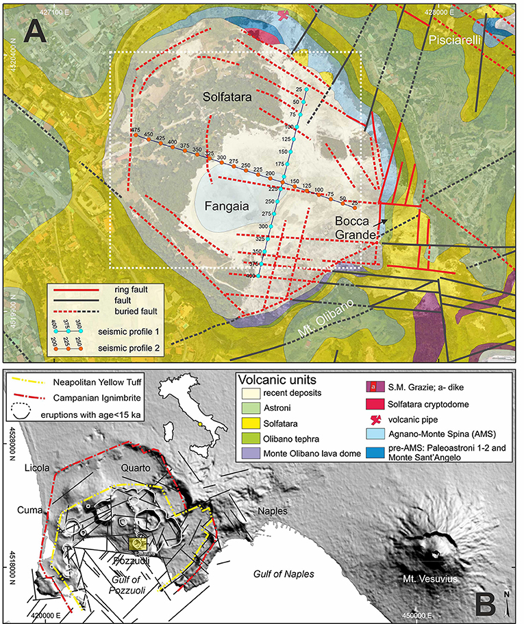
Figure 1. (A) Geological and structural map of Solfatara area (Isaia et al., 2015) overlain to a 2D image of the area (© 2019 Google); in red are the ring faults while in green are the tectonic faults; buried faults are represented by dashed lines. The white dashed rectangle shows the locations of the surface geophysical and geochemical measurements (see Figure 2). (B) DEM image showing the relationships of Solfatara (yellow-filled rectangle) with CF caldera and Somma-Vesuvius. The structural framework of Campi Flegrei Caldera is from Orsi et al. (1996), Vitale and Isaia (2014). Regional faults are inferred by geophysical studies and morphological structures (Florio et al., 1999; Milia et al., 2000; Bruno et al., 2003; Sacchi et al., 2009).

Solfatara is located ~1.2 km to the east of Pozzuoli town (Figure 1). The volcano formed during the most recent epoch of volcanic activity at Campi Flegrei at ca. 4200 yr B.P. (Isaia et al., 2009; Smith et al., 2011), which was dominated by explosive activity, mainly in the central-eastern caldera sector, climaxing with the Plinian eruption of Agnano-Monte Spina (De Vita et al., 1999) at ca. 4.5 ka. The Solfatara eruption was preceded and followed by explosive eruptions from nearby centers (Astroni, Mt. Olibano, S-M- Grazie, Agnano-Monte Spina, and pre-Astroni) whose products are found in the area around the present crater rims (Figure 1).

Geophysical, geochemical and geological data allow to infer, with different resolution and degree of uncertainty, the structure and stratigraphy of the upper part of the crater, together with the main features of the upper part of its complex hydrothermal system, made up of a mix of uprising magmatic fluids and meteoric water. High-resolution seismic reflection profiles (Bruno et al., 2017), show a ~400 m deep asymmetrical crater filled by volcanoclastic sediments and rocks and carved within an overall non-reflective pre-eruptive basement pierced by intrusive bodies: their seismic data clearly show several steep and segmented collapse faults affecting the crater filling. Faults generally have normal kinematics and dip toward the crater center. Resistivity tomography surveys, combined with mappings of diffuse CO₂ flux, ground temperature and self-potential (Byrdina et al., 2014; Gresse et al., 2017) delineate three shallow plume structures: two liquid-dominated conductive plumes below the Fangaia mud-pool and the Pisciarelli fumarole and a gas-dominated plume below Bocca Grande fumarole. In the shallow steam-heated part of Solfatara crater, a predominant argillitic alteration occurs, where sulfuric acid is created at, or above, the water table by the oxidation of H₂S (Rye, 2005). The hydrothermal activity at the surface is characterized by an intense soil diffuse degassing, both inside and outside of the crater (Cardellini et al., 2017 and reference therein). Acidic (pH ~1.7) high-temperature (≥ 160°C) fumaroles are mainly located in the eastern part of the crater, whereas hot springs, steam-heated pools (45–95°C), and fumarolic vents are concentrated in its center (Glamoclija et al., 2004; Valentino and Stanzione, 2004; Chiodini et al., 2011). The absence of vegetation (Figure 1A) best depicts the area of diffuse soil degassing.

Materials and Methods

Datasets and Integration

As briefly outlined before, we use three different multivariate datasets in this paper. The first is made of three co-located spatial geophysical and geochemical data shown in Supplementary Figure 1 and whose acquisition and processing is discussed in detail in Bruno et al. (2007). Specifically, we had four data available: (a) the high-resolution Bouguer anomaly; (b) the log₁₀ of the CO₂ flux; (c): the soil temperature; and (d): the mean environmental seismic noise level measured within the 10–15 Hz frequency window on the amplitude spectrum. However, Supplementary Figure 1 shows that both the CO₂ flux and the soil temperature bear the same type of information: i.e., temperature anomalies at Solfatara are generated by diffuse degassing of hot CO₂ gas through soil. Therefore, we decided to remove one of the two datasets (i.e., soil temperature) before clustering to avoid assigning a higher “a priori” weight to the high-temperature degassing phenomenon with respect to the other parameters.

The second, bi-variate, dataset is made by merging the shallow P-wave velocities estimated by Bruno et al. (2017) from the tomographic inversion of the first-arrival traveltimes (SRT) with the electric resistivity (ERT) estimated by Gresse et al. (2017) from the inversion of Wenner/Schlumberger profiles that are in part overlapping with the two seismic arrays. For both ERT and SRT images the co-located grid has the same progressive of the seismic dataset (Figure 1). The tomographic and electric profiles are shown in Supplementary Figures 2, 3. Electric resistivity and p-wave velocity do not show evident correlations.

The third dataset is made of four seismic attributes (Supplementary Figures 4, 5). Similarity, energy and dip attributes are computed and described by Bruno et al. (2017), on the depth-converted CRS stacks along the two profiles of Figure 1. We merged them with a new attribute (GLCM texture: see Haralick et al., 1973), computed with a step out nr = 3 and using a GLCM size of 32 × 32. All four chosen attributes were computed using a depth gate of 10 m. The energy attribute is a measure of reflectivity strength within the chosen depth-gate, while similarity is a multi-trace attribute that returns trace-to-trace similarity properties. It ranges between 0 and 1: a similarity of 1 means that the trace segments are identical in waveform and amplitude. Similarity is the best indicator of structural discontinuity: faults and fractures are generally visible as narrow low-similarity areas. The dip-angle attribute provides the apparent angle of dip (in degree) of seismic features within the profiles. The dip angle is computed from the dip-steering process that produces a steering cube, i.e., a volume that stores information about the seismic dip of coherent events at every sample position. Finally, the entropy attribute is part of the Texture-Directional attributes. This class of attributes uses the gray level co-occurrence matrix (GLCM) and its derived attributes are tools for image classification that were initially described by Haralick et al. (1973). The GLCM entropy attribute measures the disorderliness (or roughness) of the patch of seismic amplitude values; maximum entropy occurs when all probabilities of values are equal and therefore result in a random distribution of values (Malleswar et al., 2010).

The four seismic attributes described above were chosen among many possible others with the aid of Principal Component Analysis (Abdi and Williams, 2010; Kassambara, 2017), a preliminary analysis needed, for assessing the most representative attributes to use for the subsequent processing. Principal component analysis represents a rotation of the multi-dimensional point cloud so that the maximum variability is projected onto the pair-wise combination of axes (Prasad et al., 2005). The contribution of attributes and their quality were evaluated in the correlation circle (Abdi and Williams, 2010), shown in Supplementary Figure 6. Energy and similarity showed a better representation on the compared principal component, while dip angle showed the lowest values. However, the calculated values do not differ so much to justify the exclusion of dip angle from the analysis. The variances for the first two dimensions are respectively 34.7 and 29.1% (Supplementary Figure 6), their ratio is equal to 1.19, and following Kohonen (2014) these values were used to create the neural networks.

All processing steps were performed using algorithms written in MATLAB^® and R^®. As first preprocessing step, we removed from the three dataset those measurements that were outside the overlapping areas; then overlapping datasets were interpolated and resampled over a common grid. Many different approaches can be chosen for this step. For example, to avoid a loss of data to preserve the information content of both models Bedrosian et al. (2007), interpolated a 2D magnetotelluric and seismic dataset using the grid dimension of the higher-resolution data. For the tri-variate spatial dataset we followed a similar approach: we obtained a 50 × 50 square matrix (see Figure 1, dashed box) with an individual cell-size of 10 × 8.6 m. For the bi-variate (Vp, ρ) dataset, ERT and SRT were sampled with a uniform grid spacing of 3 × 3 m, a compromise between the more resolved SRT and the less resolved ERT. The 4D seismic attributes were instead exported from OpenDtect with a common depth sampling of 1 m and spatial sampling of 1 CDP (i.e., 1 m). Seismic attributes were limited to a depth of 600 m below the datum (i.e., 97 m a.s.l.) instead of the original 800 m because very few seismic features of interest are within the 600–800 m depth range. We obtained therefore two very dense four-dimensional matrices sampled along grids of 372 × 600 nodes for Profile 1 and 451 × 600 nodes for profile 2.

Since the geophysical and geochemical measurements have different ranges and standard deviations, then one dataset might dominate the distance used in clustering. Therefore, some preliminary data standardization is necessary. We used a technique known as “data sphering” (Koivunen and Kostinski, 1999), a linear transformation that converts a vector with known covariance matrix into a set of new variables whose covariance is the identity matrix, meaning that they are uncorrelated and each one has a variance of 1. For each multidimensional matrix discussed above, the p-dimensional sample mean $\bar{x}$ $\bar{x}$ and the covariance matrix S were computed, and finally, the data were sphered using the following transformation (Martinez and Martinez, 2005):

\begin{array}{l} Z_{i} = Δ^{\frac{1}{2}} Q^{T} (x_{i} - \bar{x}); & (1) \end{array}

$\begin{array}{l} Z_{i} = Δ^{\frac{1}{2}} Q^{T} (x_{i} - \bar{x}); & (1) \end{array}$

where Q are the eigenvectors obtained from the covariance matrix S, Δ is a diagonal matrix of corresponding eigenvalues, x_i is the i-th sample for any geophysical variable and x_m is its average value. Z_i is the new scaled multivariate dataset suitable as input for data mining processing.

K-Means Clustering

The K-means (Lloyd, 1982), is an unsupervised method used in data exploratory analysis to find similar observations. K-means is a partitional, non-hierarchical and unsupervised clustering algorithm, which allows separating a dataset in “k” clusters based on distances among points. The objective function of the algorithm is to minimize the within-cluster variance and to maximize it among different clusters. The within-class scatter matrix, S_w, is defined as Martinez and Martinez (2005):

\begin{array}{l} S_{w} = \frac{1}{n} \sum_{j = 1}^{m} \sum_{i = 1}^{n} I_{i, j} (x_{i} - \bar{x}) {(x_{i} - \bar{x})}^{T}; & (2) \end{array}

$\begin{array}{l} S_{w} = \frac{1}{n} \sum_{j = 1}^{m} \sum_{i = 1}^{n} I_{i, j} (x_{i} - \bar{x}) {(x_{i} - \bar{x})}^{T}; & (2) \end{array}$

where I_{i, j} is one if x_i belongs to group j and zero otherwise, and m is the number of groups. The criterion that is minimized in the K-means is the sum of the diagonal elements of S_W. Everitt and Dunn (2001) show that minimizing the sum of the diagonal elements of S_W is equivalent to minimizing the sum of the squared Euclidean distances between the individual elements x_i and their group mean.

In general, the algorithm is initialized by randomly defining an initial number “K” of centroids and assigning each observation to its closest centroid using the Euclidean distance between the observation and the cluster centroid. The second step of the procedure is to calculate the new centroids (i.e., the new mean values) using the assigned observations. These steps are repeated until there are no changes in cluster membership or until the centroids do not change (Späth, 1980).

Like many other types of numerical minimizations, the algorithm may converge into a local minimum. This often depends on the initial choice of the centroids. To choose the initial centroids based on the data, we initialized the algorithm performing a preliminary clustering on a random 10% subsample of the entire dataset, with the option “start” and “cluster”. Moreover, MATLAB's “kmeans” function allows the use of the parameter “Replicates” to overcome the above-mentioned problem of falling into a local minima. Setting a parameter higher than one in “Replicates” instructs the algorithm to begin from a different set of initial centroids, therefore, even if sometimes “kmeans” finds more than one local minimum, the final solution that the function returns is the one with the lowest total sum of distances, over all replicates. We used 20 replicates for our analysis as it was the minimum number that returned the same final results.

Another issue with the K-means algorithm is that the choice of the number of clusters, K, is arbitrary, meaning that the optimal number K has to be found using some statistical criterion. Many tools have been used in assessing the quality and optimal number of clustering as well as the degree with which a clustering scheme fits a specific data set (Halkidi et al., 2001); each tool has its own advantages and disadvantages. To assess both the optimal number K and the degree with which our clustering scheme fits our specific data sets, we used the Silhouette Index (SI: Kaufman and Rousseeuw, 1990; Brock et al., 2008). The silhouette index compares the distances of every i-th observation within a cluster with the average extra-cluster distances. In other words, the silhouette index measures the degree of confidence in the clustering assignment of a given observation. For an observation i, the silhouette index is defined as Rawashdeh and Ralescu (2012):

\begin{array}{l} S I_{i} = \frac{(b_{i} - a_{i})}{m a x (a_{i,} b_{i})}; & (3) \end{array}

$\begin{array}{l} S I_{i} = \frac{(b_{i} - a_{i})}{m a x (a_{i,} b_{i})}; & (3) \end{array}$

where: a_i is the average dissimilarity of i to all other observations in its own cluster and b_i is the minimum value of all average dissimilarity of i to all observations in any other cluster c. The average silhouette index is found by averaging SI_i over all observations:

\begin{array}{l} \bar{S I} = \frac{1}{n} \sum_{i = 1}^{n} S I_{i}; & (4) \end{array}

$\begin{array}{l} \bar{S I} = \frac{1}{n} \sum_{i = 1}^{n} S I_{i}; & (4) \end{array}$

The silhouette index in Equation 3 ranges from −1 to 1. Values <0 and close to 1 mean that the observation is well-matched to its own cluster, values near to 0 highlight observations with unclear assignment (either to the current cluster or to the nearest one), while values <0 are typical of misclustered observations. Compared with the R-Squared index (Sharma, 1996), which reveals the optimal clustering at the “knee,” the silhouette index provides less chances to choose the wrong number of clusters: this happens because finding the “knee” in noisy data is not as obvious as it could appear. While using the silhouette index, the optimal number of clusters K is where the average silhouette index (Equation 4) reaches its maximum value.

Therefore, not only the silhouette index allows evaluating the optimal number of cluster but also it provides an assessment of cluster membership. We used a hard-clustering technique for our K-means analysis, meaning that each measurement can belong only to one cluster. A hard-clustering representation in the original space shows all observations belonging to the same cluster with the same color. Therefore, transactions among clusters are graphically represented by color changes. However, to account for uncertainty in cluster membership we merged the results of the silhouette index with the K-means by saturating the color of each single measurement according to its SI. This technique is similar in principle to the technique applied by Paasche et al. (2010), where the color saturation of their images is also based on a membership function.

Self-Organizing Maps

Self-Organizing Maps (SOM) are a type of neural network suitable for unsupervised learning (Kohonen, 1997), that uses a competitive learning strategy. The SOM transforms a feature vector of arbitrary dimension drawn from the given feature space into a simplified, generally two-dimensional, discrete map (Klose, 2006). This is achieved in a manner that neurons physically located close to each other in the output layer of the SOM have similar input patterns (Kalteh et al., 2008). The SOM network preserves the original topology and delivers an intuitive visual representation of the clustering; the mapping produced by SOM is usually of the type many-to-one, i.e., the projection images on the SOM are local averages of the input data, which is comparable to the K-means averages (Gersho, 1982; Gray, 1984).

A SOM neural network is structured in two layers: an input layer and a Kohonen layer. In most applications the Kohonen layer represents a structure with a single two-dimensional map consisting of neurons arranged in rows and columns. Each neuron of the Kohonen layer is fixed and is fully connected with all source neurons in the input layer. The input variables, can be represented as vectors of the type ${\vec{x}}_{} = {x_{1}, x_{2}, x_{3}, \dots x_{n}}^{T}$ ${\vec{x}}_{} = {x_{1}, x_{2}, x_{3}, \dots x_{n}}^{T}$ in the space Rⁿ where n is the dimension of the input space (Wehrens and Buydens, 2007). In our case, the vector space n has four-dimensions (i.e., the four seismic attributes used for our analysis). The objective of the algorithm is to organize the input seismic attributes into a geometric structure. If the map has q neurons there are q prototype vectors, or weights, defined as:

\begin{array}{l} {\vec{ω}}_{k} = {ω_{(k, S),} ω_{(k, E),} ω_{(k, D),} ω_{(k, H),}}^{T} & (5) \end{array}

$\begin{array}{l} {\vec{ω}}_{k} = {ω_{(k, S),} ω_{(k, E),} ω_{(k, D),} ω_{(k, H),}}^{T} & (5) \end{array}$

Where: S is the Similarity attribute, E is the Energy, D is the Dip, H is the Entropy and K = 1,2,…., q. The codebook vectors are initialized as random values. ${\vec{ω}}_{k}$ ${\vec{ω}}_{k}$ connects the n input layer neurons to the total number of neurons q in the Kohonen layer. Learning occurs during the self-organizing procedure as the input vectors ${\vec{x}}_{} = {S, E, D, H}^{T}$ ${\vec{x}}_{} = {S, E, D, H}^{T}$ are presented to the input layer of the network. The weights ${\vec{ω}}_{k}$ ${\vec{ω}}_{k}$ are used to determine only one stimulated neuron in the Kohonen layer after the “winner-takes-all” principle that can be summarized as follows: for each $\vec{x}$ $\vec{x}$ , the Kohonen neurons compute their respective values of a discriminant function (i.e., Euclidean distance ( $| | {\vec{x_{i}}}_{} - {\vec{ω}}_{k}_{} | |$ $| | {\vec{x_{i}}}_{} - {\vec{ω}}_{k}_{} | |$ ). These values are used to define the winner neuron. That means the network determines the index j of that neuron, whose weight ${\vec{ω}}_{k}$ ${\vec{ω}}_{k}$ is the closest to vector $\vec{x_{i}}$ $\vec{x_{i}}$ by:

\begin{array}{l} j (\vec{x_{i}}) = a r g m i n ‖ {\vec{x_{i}}}_{} - {\vec{ω}}_{k}_{} ‖ | k = 1, 2 \dots, m, \dots q & (6) \end{array}

$\begin{array}{l} j (\vec{x_{i}}) = a r g m i n ‖ {\vec{x_{i}}}_{} - {\vec{ω}}_{k}_{} ‖ | k = 1, 2 \dots, m, \dots q & (6) \end{array}$

Afterwards, the learning procedure modifies the weights ${\vec{ω}}_{j}$ ${\vec{ω}}_{j}$ of the winner neuron and the winner neighborhood.

\begin{array}{l} {\vec{ω}}_{k} (t + 1) = {\vec{ω}}_{k} (t) + η (t) \cdot h_{k, j (\vec{x_{i}})} (t) \cdot [\vec{x_{i}} {(t)}_{} \\ - {\vec{ω}}_{k} {(t)}_{}]; & (7) \end{array}

$\begin{array}{l} {\vec{ω}}_{k} (t + 1) = {\vec{ω}}_{k} (t) + η (t) \cdot h_{k, j (\vec{x_{i}})} (t) \cdot [\vec{x_{i}} {(t)}_{} \\ - {\vec{ω}}_{k} {(t)}_{}]; & (7) \end{array}$

where t denotes the iteration number, η(t) is the learning-rate parameter during the calculation step t, and $h_{k, j (\vec{x_{i}})}$ $h_{k, j (\vec{x_{i}})}$ is the neighborhood function centered around the winning neuron $j (\vec{x_{i}})$ $j (\vec{x_{i}})$ . The learning rate η(t) is usually a small value in the order of 0.05, which decreases during the training so that the map converges. The size of the neighborhood function also decreases during training and eventually only the winning units are modified (Wehrens and Buydens, 2007). Thus, the codebook vectors are updated at each iteration and the algorithm terminates after a predefined number of iterations.

The initialization parameters have their importance, because also the SOM, as for the K-means, can get trapped in a local minimum solution. As for the K-means, repeated training of a SOM will lead sometimes to a rather different mapping, because of the random initialization. However, the conclusions drawn from the map remain remarkably consistent among different initialization of the same data, which makes the SOM a very useful tool in many circumstances (Wehrens and Buydens, 2007).

The initialization parameters (such as the grid size and the number of iterations) are important to a successful SOM analysis. As recommended by Vesanto and Alhoniemi (2000), the grid should have a number of nodes well above the number of real clusters in the dataset. One may have to test several grid sizes to check if the cluster structures are shown with a sufficient resolution and statistical accuracy (Kohonen, 2014). To define the shape of the map we need to compute the first two principal dimensions in which the variances of the input dataset are. The ratio between the number of neurons in the two directions of the grid is proportional to the ratio between the two principal components (Kohonen, 2014). Here, following Abdi and Williams (2010), we assessed the quality of the representation of the variables on the factor map by using the “square cosine, squared coordinates” (i.e., cos²) method. A high cos² highlights a good representation of the variable on the principal component (i.e., the variable is close to the circumference of the correlation circle). A low cos² suggests that the variable is not perfectly represented by the principal components (i.e., it is close to the center of the circle).

The nets sizes used by us were computed taking into account the ratio of the number of neurons according to the following formula (Kohonen, 2014):

\begin{array}{l} R = \frac{v a r 1}{v a r 2} ≅ \frac{n 1}{n 2} & (8) \end{array}

$\begin{array}{l} R = \frac{v a r 1}{v a r 2} ≅ \frac{n 1}{n 2} & (8) \end{array}$

where var1 and var2 are the variance for the first and second principal component respectively, while n1 and n2 are the number of neurons along the x and y directions of the neural network. The relationship between the neurons constituting the two dimensions of the network is derived from the ratio of variance between the first two principal components. Through Equation 8 therefore, we determine the value of n1 by imposing n2. Differently from the empiric approach proposed by several authors (e.g., Céréghino and Park, 2009), where sizing of a neural network is based on the number of observations constituting the multivariate dataset, we prefer to use a smaller number of neurons but significantly greater than the number of expected seismic facies. The optimal size of the network is identified by successive attempts, using Equation 8, and increasing the number of neurons until we obtain a SOM image that best represents the expected geophysical/geological features. Our approach allows to represent all neurons in the network with a different color, through a color map based on the position of the neurons as discussed below. Differently from Céréghino and Park (2009), our approach allows shorter computation times and preserve all the details, avoiding a possible loss of information due to the need (in order to have a coincise representation of the starting space) of grouping together the high number of neurons, often resulting from the empirical approach of Céréghino and Park (2009). In fact, Unglert et al. (2016), show that the clustering process applied to the SOM results may fail to regroup the neurons in a manner that is consistent with the input dataset presented to the SOM.

With the aim to allow the neural network to replicate the topological distribution of the dataset, we presented it to the SOM 9,000 times. We inspected the training progress by checking the average distance of an object with the closest codebook vector (Wehrens and Buydens, 2007). Moreover, for the neurons a hexagonal connectivity was adopted resulting with a number of six neighbors for the inner neurons, with a planar topology for the lattice.

Displaying SOM Maps

Once the SOM algorithm has converged, the two-dimensional feature maps of Kohonen neurons display the following important statistical characteristics of the represented feature space (Klose, 2006):

Approximation: A feature map represented by a set of weights in the Kohonen layer provides a good approximation to the input space. Topological ordering: The two-dimensional feature map is topologically ordered in the sense that similar Kohonen layer neurons correspond to similar feature vectors of the higher dimensional input space. Density matching: The feature map reflects variations in the statistics of the distribution of the original feature space: regions in the input space from which sample vectors are drawn with a high probability of occurrence are mapped onto larger domains in the Kohonen layer, and therefore with better resolution than regions in the input space where sample vectors are drawn with a low probability of occurrence.

Since the SOM preserve the topological ordering of the input space (i.e., similar input features are classified within the same neuron or within adjacent neurons) it makes sense to display the results using a color map based on the relative position of neurons. The most used method to visualize the cluster structure of a SOM is based on the unified distances matrix (U-matrix; Ultsch, 1993). This is a visualization technique that allows to represent the structural properties of the high dimensional input space with a color scale based on the relative distance between the prototype vectors and the winner unit and it is conceptually similar to the gradational color scales used to represent data from digital elevation models. A synoptic view of the input multivariate dataset is also needed for result interpretation, to identify features across the neurons and highlight correlations that in our case could be interpreted as signatures of hydrothermal features. Here we adopted the “heatmaps” (see Pryke et al., 2007) as a way to represent the average values of input observations classified into each neuron. The heatmaps, computed by averaging the variables classified into each neuron, are powerful ways to show the distribution of the different variables (i.e., seismic attributes) across the neural network, thus facilitating a visual interpretation of the classification provided by the SOM. The variable range is represented by a gradational color scale, in which we assign cold colors to the lowest values and hot colors for the highest values (Supplementary Figure 7).

The method we propose to graphically represent distances between neurons uses a RGB color gradation based on both the position of neurons and on the values of U-matrix, to consistently image input seismic facies in the original space in the output 2D lattice (Supplementary Figure 7A). The x,y neuron coordinates in the 2D lattice provide the R and G values while the U-matrix value provides the B value. All RGB values are scaled to fit the range from 0–255. This RGB color map will show similar colors for adjacent neurons, while the B U-matrix value is useful to highlight distances of neurons, showing how far are the observations. This method is analog to the coloring scheme used by Langer et al. (2009) with the difference that Langer et al. (2009) did not use the U-matrix value in coding the RGB colors.

Results

Surface Data Integration

The results obtained by K-means on the tri-variate dataset composed by the Bouguer anomaly, CO₂ flux and seismic noise are in Figure 2. The optimal cluster number, assessed by the silhouette index is K = 4 (Figure 3). Light colored pixels are those characterized by a low silhouette index and therefore of uncertain collocation between adjacent clusters. Misclustered pixels (i.e., SI <0) are colored in white. The clusters boundaries show a prevailing NE and WNW trend and an excellent agreement with the patterns of the intracrateric tectonic structures mapped by Isaia et al. (2015). This agreement clearly demonstrates that the surface distribution of the analyzed geophysical and geochemical data, which reflects the undergoing hydrothermal activity at Solfatara, is mainly influenced by the tectonic framework. This evidence is clearer on the outcomes of the cluster analysis (Figure 2) rather than on the individual measurements of Supplementary Figure 1.

FIGURE 2

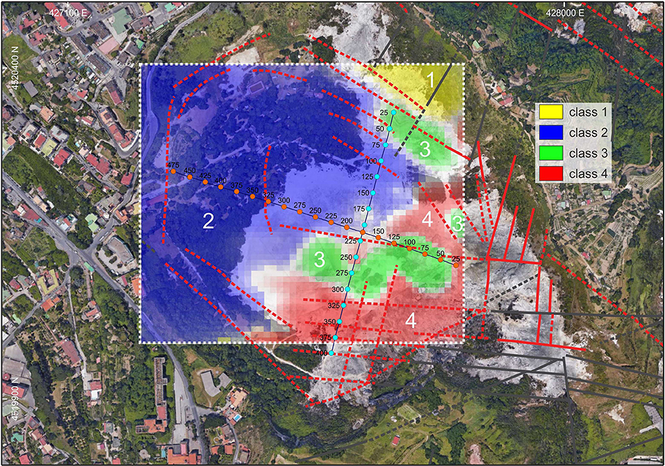
Figure 2. 2D image of the Solfatara area (© 2019 Google) as in Figure 1 with results of surface dataset integration by means of K-means clustering overlaid with the main faults from Isaia et al. (2015). Dots in light blue are the CDP metrics of Profile 1 while dots in orange are the CDP metrics of Profile 2.

FIGURE 3

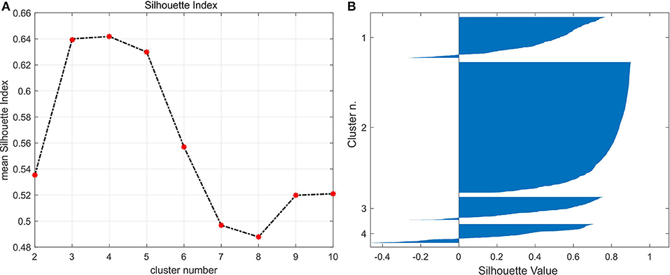
Figure 3. Validation of K-means clustering analysis of the surface dataset with the Silhouette index. (A) Silhouette index showing a maximum average value for k = 4; (B) graphical Silhouette values for each cluster of the k = 4.

Supplementary Figure 1 overlays the hard cluster partitioning obtained by the K-means analysis to the spatial distribution of the three variables used for the clustering (plus the soil temperature, which was not included in the analysis). A qualitative assessment of the average value of each variable in each of the four clusters is reported in the Table 1.

TABLE 1

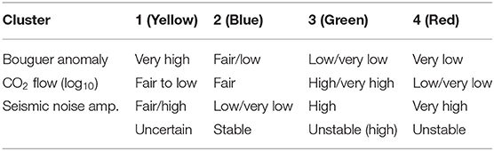
Table 1. Qualitative average values of Bouguer anomaly, CO₂ flow and Seismic noise amplitude in each of the four clusters.

Cluster 2 (in blue in Figure 2) has the largest surface extension and it is overall characterized by low values of the three analyzed variables. It highlights the most stable sector of Solfatara not much affected by the hydrothermal dynamics. Vice-versa the most active areas (such as the “Fangaia” and the “Stufe di Nerone” fumaroles) are highlighted by cluster 3 (green), which combines high values of CO₂ flow and seismic noise with low values of the Bouguer anomaly. Cluster 3 most likely emphasizes the surface location of the main degassing pathways.

Cluster 4 (red) alternates spatially with cluster 3 and is characterized by low- to very-low values of Bouguer anomaly and of CO₂, which it is considered to be, together with the surface temperature, the main indicator of magmatic degassing, and by the highest values of seismic noise. In general, the high levels of seismic noise characterizing both clusters 3 and 4 can be associated with the intense vibrational activity connected with the uprising fluxes.

Finally, cluster 1, characterized by very high values of Bouguer anomaly and average values of the other two variables, has the smallest extension and it is only found in the NE corner of the investigated area, close to the Solfatara cryptodome and to a volcanic pipe (Figure 1). The high bouguer anomaly within cluster 4 can be therefore by explained by a higher rock density of the crater rims with respect to the volcanoclastic material filling the crater.

Near-Surface Resistivity and P-Wave Velocity Integration

The clustering of the electrical resistivity and the P-wave seismic tomography along the two profiles shown in Figure 1 was done with the purpose of assessing the hydrological properties (i.e., gas-saturated vs. water saturated porous media and degree of saturation) of the near surface, since both the electrical resistivity and the P-wave velocity are sensitive to changes of water/gas saturation. The analysis of the silhouette index revealed that the optimal number clusters is consistently 3 for both Profile 1 (Figure 4) and Profile 2 (Figure 5). Moreover, both the cross-plots in Figures 4B, 5B show that three clusters are well-separated. As for the previous analysis we report in the Table 2 a qualitative assessment of the average value of each variable in each of the three clusters.

FIGURE 4

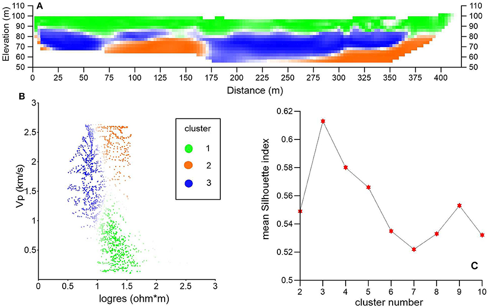
Figure 4. Results of integration based on the K-means analysis for the bi-variate dataset composed of ERT and SRT on Profile 1. (A) Integrated image with three clusters and saturated with the Silhouette index. (B) Bi-variate dataset in the joint parameter space with colors saturated with the Silhouette index. (C) Optimal clustering for k = 3 highlighted by the maximum value in k = 3.

FIGURE 5

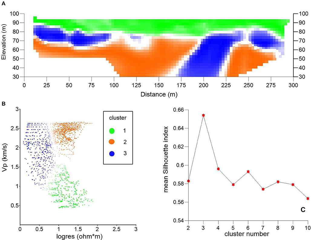
Figure 5. Results of integration based on the K-means analysis for the bi-variate dataset composed of ERT and SRT on Profile 2. (A) Integrated image with three clusters and saturated with the Silhouette index. (B) Bi-variate dataset in the joint parameter space with colors saturated with the Silhouette index. (C) Optimal clustering for k = 3 highlighted by the maximum value in k = 3.

TABLE 2

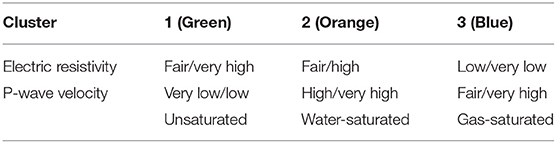
Table 2. Qualitative average values of electric resistivity and P-wave velocity in each of the three clusters.

In both cross-plots, cluster 1 (in a green color) combines low values of P-wave velocity with fair to very high values of electric resistivity. These values are typical of loose, unsaturated to partly saturated tephra affected by diffuse CO₂ degassing therefore confirming the findings of Chiodini et al. (2001), Bruno et al. (2007, 2017), and Gresse et al. (2017). As it can be seen in both Figures 4A, 5A, cluster 1 occupies the topmost part of both profiles for an average thickness of 10–30 m. Clusters 2 (orange) and cluster 3 (blue) are both characterized by a fair-to-very high P-wave velocity (higher for cluster 2) but while cluster 3 has very low values of resistivity, cluster 2 is instead characterized by a higher resistivity. We tentatively associate cluster 2 with predominantly gas-saturated porous media and cluster 3 with predominantly water-saturated porous media. P-wave velocity should decrease in the presence of gas: therefore, high-values of P-wave velocity in cluster 2 are a bit odd and can be explained hypothesizing an overall high-water saturation (i.e., presence of a two-phase fluid) even in the predominantly gas-saturated area. Both clusters are found at depths <10–30 m in the integrated images in Figures 4A, 5A.

Seismic Attribute Integration

Seismic attributes were integrated using both the K-means and SOM techniques. For the K-means clustering, the mean Silhouette Index indicates an optimal value of 7 clusters (Figure 6), for which we qualitatively assess the average ranges of each of the four seismic attributes in Table 3. The subsurface 7-cluster distribution can be observed in Figures 7, 8, where we can also compare the results between SOM and K-means. For example, on both profiles (Figures 7, 8) and on the depth range 250–450 m cluster 1 (red) highlights elongated features characterized by high to very high entropy, dip and similarity that can be interpreted as intrusive bodies (dikes). Instead, only on profile 1 and in a shallower (100–300 m) depth range, cluster 5 (beige) and to a lesser extent cluster 4 (yellow) and 1, show some peculiar sub-vertical thin patterns that cross-cut or are found below areas belonging to cluster 2. These features are not evident with the same clearness on Profile 2 (Figure 8) because, as discussed in Bruno et al. (2017), this profile is characterized by a lower S/N ratio possibly correlated to a higher structural complexity of the Solfatara along the WNW-ESE direction (Isaia et al., 2015). In both profiles, clusters 2 (dk green) and 7 (purple) highlight sub-horizontal structures with high energy and similarity. Cluster 3 (green) features areas overall characterized by high-reflectivity in profile 1 while it is not discriminant of any facies in profile 2, due to lower S/N ratio. Cluster 3 and 6 (lt. green) have similar average values, however in profile 1 cluster 3 has a spatial distribution that highlights the upper filling of the crater down to a depth of ~350 m.

FIGURE 6

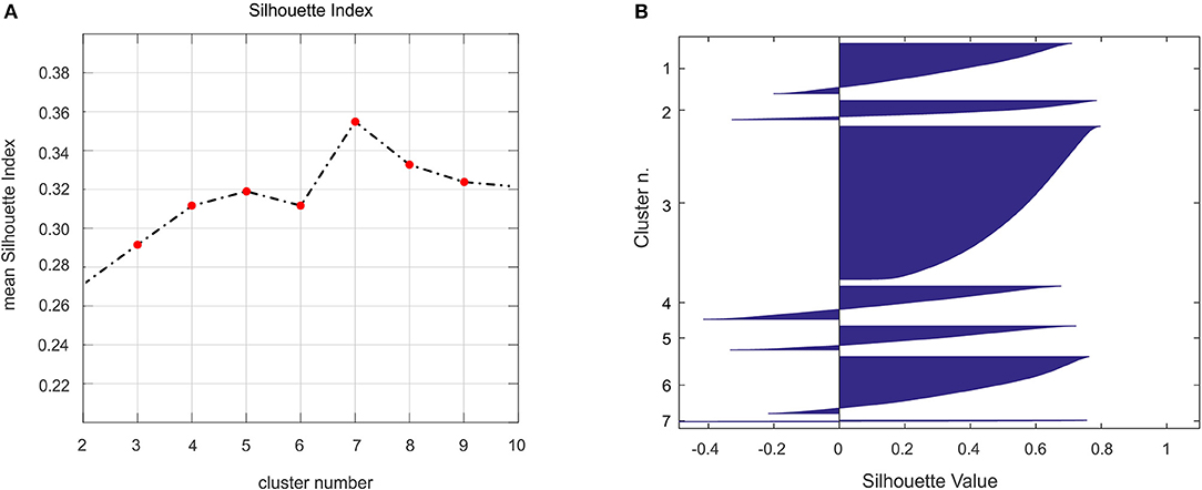
Figure 6. (A) Mean silhouette index obtained after K-means clustering of the seismic attributes varying the number of clusters from 2 to 10. The optimal clustering was found at the maximum value for k = 7; (B) graphical Silhouette values for each cluster of the k = 7.

TABLE 3

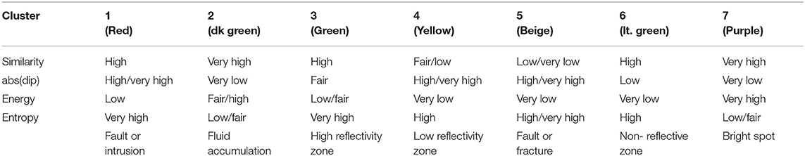
Table 3. Qualitative average values of similarity, abs(dip), energy, and entropy in each of the seven clusters.

FIGURE 7

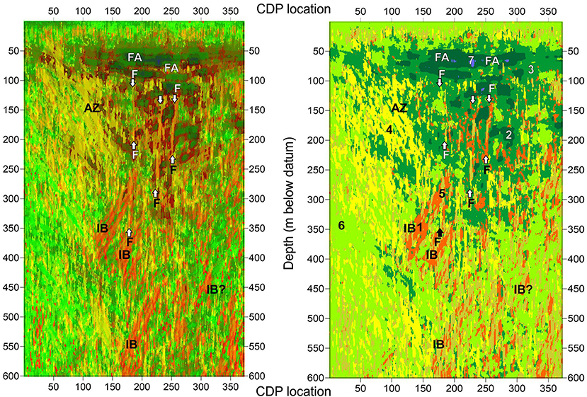
Figure 7. Seismic attribute integration along profile 1. Left image obtained with SOM. Right image obtained with K-means. In the right image the seven clusters labeled by numbers: 1, red; 2, dark green; 3, green; 4, yellow; 5, beige; 6, light green; 7, purple 3. Symbol explanations. AZ, asymmetric zone; F, fault/fracture (also highlighted by vertical arrows); FA, fluid accumulation; IB, intrusive body.

FIGURE 8

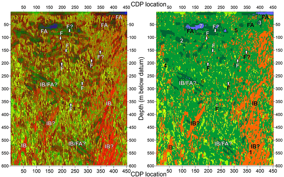
Figure 8. Seismic attribute integration along profile 21. Left: image obtained with SOM. Right: image obtained with K-means. In the right image the seven clusters labeled by numbers: 1, red; 2, dark green; 3, green; 4, yellow; 5, beige; 6, light green; 7, purple 3. Symbol explanations. F, fault/fracture (also highlighted by vertical arrows); FA, fluid accumulation; IB, intrusive body.

As discussed above, we also performed the SOM analysis on the seismic attribute datasets using different neural networks with increasing size (6 × 5, 8 × 7 and 12 × 10 nodes). The 12 × 10-node network provided the best details in the integrated images for both profiles 1 and 2. Those node maps are also shown in Figures 7, 8 and overall display more consistent results and better details than the corresponding K-means images. As explained before, in order to reflect the distribution of attributes across the lattice, the SOM results are displayed by using an RGB colormap based on the geometry of the neural network and on the U-matrix values. By matching the SOM and K-means images and by a synoptic comparison of RGB colormap (Supplementary Figure 7A), heatmaps (Supplementary Figures 7C–F) and K-means clusters of the two integrated profiles (Figures 7, 8) five main volcanic/hydrothermal facies could be inferred. These facies include all the 120 SOM neurons of Supplementary Figure 7A.

Facies 1 groups neurons 1–4, 13–16, 25–27, 37–39, 49–50 in Supplementary Figure 7A, and roughly corresponds to cluster 2 (i.e., dark green) and 7 (i.e., purple) of the K-means analysis. Such facies is characterized by fair to very high energy, very high similarity, very low values of entropy and by sub-horizontal dips (see Supplementary Figures 4, 5) and is visible on Profiles 1–2 as sub-horizontal to slightly dipping, dark-colored zones in the depth range 50–300 m on the two profiles (Figures 7, 8). We interpret them as sub-horizontal areas of fluid (both gas and water) accumulation within the crater.

Neurons n. 57–59, 69–72, 82–84, 96, 106–108 in Supplementary Figure 7A, with high dip, very low energy, high entropy and low similarity, are instead grouped into Facies 2. Such facies includes cluster 5 and in part 1 and 4 of the K-means analysis. Neurons here show characteristic sub-vertical thin patterns and are interpreted as narrow, faults/fractures filled with fluids of hydrothermal origin. They are extremely well evident at CDP 100–300 and at depths of 100–500 on the image of profile 1 (Figure 7A).

Facies 3 groups neurons 81, 94, and 95 that have fair to low energy, high right-dip and entropy and fair similarity and are mainly present on the left side of the section from the depth of about 50 m up to 300 m, creating an asymmetric zone labeled as AZ (i.e., asymmetric zone) on the section of Profile 1 (Figure 7A). These features, which are comparable in part to cluster 4 (i.e., yellow) in Table 3 may represent old, low permeability faults/fractures or other dipping bodies (intrusions).

Neurons 22, 23, 33–35, 46, 47 are grouped in Facies 4, overall characterized by high dip, mainly left-dipping, fair to low similarity, low energy and fair to high entropy. This facies roughly corresponds to cluster 1 of the K-means analysis. We associate it to intrusions with high-dip angle (dykes) visible mainly in the 300–600 m depth range.

Finally, facies 5 groups instead all remaining neurons in Supplementary Figure 7A, which, in lack of well logs and other geological constraint we were unable to associate to any peculiar seismic feature. It correspond roughly to clusters 4 and 6 of the K-means analysis. In general observations colored with a light green-yellow in Figures 7, 8 have very low energy, variable dip, fair similarity and entropy and are distributed at the borders of the images.

Discussion

Results Comparison

Figures 9, 10 show two three-dimensional cross-sections of Solfatara crater along the NNE and WNW direction (i.e., profiles 1–2). With these figures we compare: (1) the K-means clustering of the surface data with (2) the K-means clustering of resistivity and P-wave velocity and (3) with the SOM analysis on seismic attributes. For the last dataset we choose to display the SOM results and not the K-means clustering because, as better explained in the following sections, the SOM results are far more informative than the corresponding K-means images, especially along profile 2.

FIGURE 9

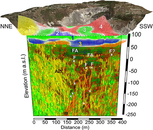
Figure 9. Three-dimensional cross-section of Solfatara crater along profile 1 showing the spatial relationships between the results of the surface data integration, overlain to the 3D topography of the Solfatara with the results of the near-surface resistivity and P-wave velocity integration and with the results of the SOM analysis on seismic attributes. Symbols explanations are as in Figure 7.

FIGURE 10

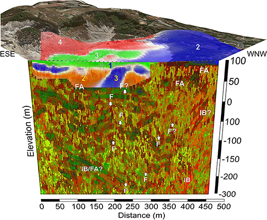
Figure 10. Three-dimensional cross-section of Solfatara crater along profile 2 showing the spatial relationships between the results of the surface data integration, overlain to the 3D topography of the Solfatara with the results of the near-surface resistivity and P-wave velocity integration and with the results of the SOM analysis on seismic attributes. Symbols explanations are as in Figure 7.

The SOM images show, at 50–350 m deep, well-definite areas of fluid accumulation (Facies 1, labeled as FA in Figures 9, 10). Bruno et al. (2017) interpret these zones as stratigraphic traps in which uprising hydrothermal fluids (both gas and water) accumulate, fed by an underlying sub-vertical network of faults and fractures (i.e., Facies 2). These faults are evident in our SOM results as narrow sub-vertical features (i.e., Facies 2) starting at depths of ~100 m (i.e., 0 m a.s.l.) and intersecting the deeper areas of fluid accumulation (e.g., FA in Figure 9). The overlain K-means analysis of resistivity/P-wave velocity allows us to discern, within the upper areas of fluid accumulation, predominantly gas-saturated media (i.e., cluster 2) and predominantly water-saturated media (i.e., cluster 3). We note that in both profiles, gas-saturated (i.e., orange) areas are found below the water-saturated (i.e., blue) zones. Overall, three main lateral heterogeneities are visible at a distance of ~60 m and ~170 m on NNE trending profile 1 of Figure 9 and at a distance of ~175–200 m on the WNW trending profile 2 of Figure 10. We argue that these lateral variations in the distribution of clusters 2–3, are controlled by fault/fractures affecting the very shallow hydrothermal circulation, Vice-versa cluster 1 (in green) which marks the unsaturated medium, does not show any significant lateral variation along the two cross-sections.

Next, we correlate the variations in the K-means clustering along the two profiles with the pattern of the surface K-means clusters within the crater (Figure 2), which we recall show an excellent agreement with the distribution of the intracrateric tectonic structures mapped by Isaia et al. (2015). In doing this comparison we need to keep in mind that the two datasets were acquired in different periods and are made of entirely different geophysical parameters (i.e., Bouguer anomaly, CO₂ flux and seismic noise amplitude vs. resistivity and P-wave velocity). Despite these facts, on profile 1 (Figure 9) we observe an overall good agreement between the patterns of subsurface and surface cluster boundaries. This agreement worsens on profile 2, probably because of its lower-S/N ratio. However, we can still notice on this latter profile that the boundary between surface clusters 3–4 (which highlight the most unstable areas of the crater) and cluster 2 (i.e., the most stable) occurs at a distance of ~200 m, above the aforementioned lateral transaction between cross-sectional cluster [2 (i.e., gas saturated) and 3 (i.e., water-saturated].

It is worth noting that the surface datasets were acquired between in 2000 and 2004 and the subsurface geophysical (i.e., seismic and geoelectrical) data were acquired on in 2014–2015. A minor lack of correlation, noticeable among the different datasets, can be therefore associated to the high dynamism of the Solfatara volcano. Anyway, the overall good agreement between the three sets of geophysical data examined with the two machine learning techniques whiteness the fact that the main shallow structural patterns, which influence the hydrothermal dynamics at Solfatara volcano, remained mainly unchanged in the last 15 years. This is not a minor outcome of this work.

K-Means vs. Self-Organizing Maps

One of the purposes of this paper was compare the performance of two machine-learning algorithms in integrating the four seismic attributes computed from the orthogonal seismic reflection profiles of Bruno et al. (2017) which are macroscopically characterized by a different S/N ratio. The two datasets have a high number of nodes (372 × 600 for profile 1 and 451 × 600 for profile 2). The process of reducing the dimensionality of the vectors, which is essentially a data compression technique, was done through SOM and K-means clustering. The idea behind both algorithms is to map high-dimensional vectors onto a smaller dimensional (typically a 2D) space (Klose, 2006). In addition to data compression, a SOM, however, creates a network that stores information in such a way that any topological relationships within the training datasets is maintained (Kalteh et al., 2008). At a more intuitive level, both K-means and SOM are moving nodes toward denser areas of the high-dimensional space. With K-means, the nodes move freely, with no direct relationship to each other. With SOM, when a node moves toward the data, it pulls neighboring nodes in the 2D lattice along with it. This naturally maintains a topology embedded in the data space. Therefore, unlike the K-means, with the SOM, vectors that are close in the high-dimensional space also end up being mapped to nodes that are close in 2D space. SOM, therefore, preserve the topology of the original data because the distances among neurons in 2D space reflect those in the high-dimensional space. However, in the case of a low number of nodes (such as our surface and near-surface data) K-means provides results very similar to SOM because it forces every vector to match an existing node, acting as a prototype/centroid, without any room for divergence. In the case of a high number of nodes, with SOM there is instead a margin for showing transitioning zones, which mimic the space among prototypes/centroids, thus modeling the transformed topological space among samples. In this way, the relative distances are “preserved” at expenses of a larger iteration time. This is a desirable feature, especially when dealing with data characterized by low S/N ratios.

Preservation of the original topological space translates into preservation of subtle features; this is evident when we compare the results of K-means and SOM with the seismic attribute datasets in Figures 7, 8 or Figures 9, 10. On profile 1, which holds a better S/N ratio, the comparison between SOM and K-means (Figure 7) shows an overall good agreement and conveys the same type of information. Therefore, even if the SOM image is more complex and detailed, when geological constraints are not available, such as in our case, the colormap simplification provided by K-means might actually help in synthesizing a simple geological interpretation. However, on profile 2 (Figure 8), which is characterized instead by a much lower S/N ratio, the preservation of the original topological space provided by the SOM results in an image that is far more informative than the K-means image. For instance, hints of possible sub-vertical faults (labeled as “F” in Figure 8), highlighted by subtle color changes on the SOM image, are totally missing on the K-means image (see the corresponding labels pointing at the exact locations in Figure 8). Therefore, in this latter profile the color map simplification provided by K-means is a flaw and SOM results hold more potential for geological interpretation.

As stated above, the coloring scheme of the SOM neural network must reflect the distribution of variables (i.e., seismic attributes) across the lattice. With our coloring scheme, based on the position of neurons and the neighborhood distances of neurons (i.e., U-matrix), nearby features have similar color gradations. One of the limits of this approach is the absence of a quantitative criteria to assess the validity of the results (de Matos et al., 2006; Roden et al., 2015); moreover, when dealing with a high number of neurons only subtle color differences characterize neighboring neurons (i.e., similar classified observation). The lack of a sharp color change in some cases makes it hard to reveal differences among observations (see again Figure 8).

Soft K-Means Clustering by the Silhouette Index

Both the tri-variate geophysical dataset measured at the surface of the crater and the bivariate tomographic dataset estimated along the two profiles are characterized by a low number of nodes. As discussed above, SOM maps with a small number of nodes are expected to behave in a way that is similar to K-means, therefore we chose the latter and faster method to analyze the above datasets. For these analyses we employed a hard-clustering algorithm but we modified the colormap of each observation by linking the Silhouette Index to the pixel color saturation as shown in Figures 2, 4A, 5A. As discussed above, the Silhouette Index ranges from −1 to 1. In our color maps light color saturations reveal clusters with values of the Silhouette Index near to 0, which highlights observations with unclear assignment. Values <0, which are typical of misclustered observations are colored in white. Our approach is therefore similar to a soft clustering (Paasche et al., 2010) and helps in reducing well-known limits of the K-means with clustering data at the edges of the clusters. Moreover, a Silhouette Index-based color map can be helpful in highlighting intra-cluster zones where geophysical parameters are changing. This improvement can provide more complete and realistic results with respect to the typical hard clustering algorithms since it allows to locate areas were observations are well/poorly clustered, spot local dissimilarities and transition zones.

Conclusions

In this work we tested the K-means and the SOM methods, widely used in multivariate clustering analysis, for the integration of different geophysical surveys acquired within Solfatara, on different scales and with different sensitivities, with the aim of providing robust geophysical models of the shallow hydrothermal system and processes. In applying these techniques, we explored two innovative approaches: for the K-means we propose to modify the color intensity of the clusters based on the Silhouette Index in order to graphically locate the membership uncertainty of the individual observations. This is useful to account for differences between observations who might be proximal or distant from their relative centroids and consequently allows us to go beyond a rigid classification which is typical of K-means clustering. This approach, detailed in the previous section, allows to visualize graphically the uncertainty of cluster assignment, which is not possible for K-means, this being a hard-clustering method. It also allows to highlight intra-cluster dissimilarities, which might indicate variability of geophysical characteristics within the same cluster number.

For the Self-Organizing Maps, we propose an alternative method for choosing the number of nodes of the neural network which aims to avoid the need for downstream clustering of the results of the classification. Our approach is based on the dimensioning of a neural network with a limited number of neurons but much greater than the dimensions of the expected seismic facies. In this way a possible loss of information is minimized with respect to larger number of nodes who have necessarily to be grouped after SOM analysis, through classic clustering techniques. Moreover, our approach makes it possible to represent all the neurons on the original space of the dataset (in our case CDPs vs. depth), by means of a color map based on: (1) the position of the neurons and (2) on the U-matrix values, maintaining all the details of the individual neurons.

Overall, our results show that both methods hold a great potential to aid an unbiased interpretation of geophysical data in complex geological settings. Similarly to other active volcanic areas, Solfatara hydrothermal dynamics leaves subtle but detectable footprints in each investigated geophysical dataset. While these hints are not easy to spot by classical interpretation schemes based on a single-method approach, their detection is highlighted by merging and compressing the vast amount of geophysical information with both the unsupervised learning methods analyzed in this paper. This is evident in Supplementary Figures 1–3 where we show the hard-cluster classification from the K-means overlain on each of the original data used for the analysis. This type of plot is very useful for post-analysis qualitative assessment of results. For instance, Supplementary Figure 1 allows us to understand that each of the three-surface datasets used provided an important contribution to clusters classification, even if the main contribution was delivered by the CO₂ flux. Similarly, Supplementary Figures 2, 3 show that the ERT data were dominant in the subsurface K-means clustering, while P-wave tomography provided a smaller contribution. Nevertheless, from a thorough analysis of those figures it is evident that unsupervised learning techniques were highly successful in synthesizing the complex geophysical information provided by each single dataset in a simpler, more meaningful model of the surface and of the shallow subsurface of the volcano. A proof of this can be found in Figure 2 that show us how well the patterns of the surface clusters correlate with the strike of intracrateric tectonic structures mapped by Isaia et al. (2015).

Another important point worth highlighting is that generally color maps used to represent the individual datasets, such as the ERT or the P-wave tomography, are subjective; i.e., their choice does influence our interpretation. In other words, by changing the colormap the resulting image changes slightly and the interpretation is affected by this change. For instance, the colormap used to represent our P-wave velocities in Supplementary Figures 2, 3 does not enhance subtle lateral variations while the colormap used to represent ERT data well-enhances them: however, by changing those color maps we could influence the interpretation of lateral and or vertical heterogeneities. This is clear by comparing the ERT and P-wave images with the overlain K-means clusters: it is impossible to determine the exact position of the cluster boundaries in an objective manner only from the ERT and P-wave images.

To further highlight the improvement in achieving objective characterization of the shallow hydrothermal system of the volcano, we use Supplementary Figures 8, 9 to show a comparison performed, across the two profiles, between the results obtained from K-means and SOM algorithms and the original seismic reflection and ERT data: it is evident the great aid provided by the unsupervised learning methods for detection of the subsurface areas of fluid accumulation and their structural pathways underneath Solfatara. For instance, while the classical interpretation schemes, based on the analysis of reflection offset and reflection strength can profitably be used on the seismic reflection data of Supplementary Figure 8 to pinpoint the location of sub-vertical faults and bright spots associated to fluids, the details provided by SOM and K-means images allows to increase our confidence in the interpretation. This support is particularly valuable when the interpreter has to deal with data at low S/N ratio, such as those shown in Supplementary Figure 9, where the results provided by machine learning algorithms on multivariate dataset can provide important constraints in minimizing the interpretation risk.

Considering that Solfatara and the neighboring areas are experiencing an new period of volcanic unrest and considering the vast amount of diverse geophysical, geochemical and geological data acquired in these area in the recent years, we hope that our case study will further promote the use of unsupervised learning techniques with the purpose of minimizing the interpretation risk and of achieving an improved understanding of the complex dynamics occurring in volcanoes.

Data Availability Statement

The datasets analyzed during the current study are freely available from the MEDSUV-RICEN website (www.med-suv.eu) and from the corresponding author on reasonable request.

Author Contributions

SB wrote MATLAB and R routines for SOM and K-means processing of the seismic attributes and of the P-wave velocity and resistivity data. PB interpreted the results, wrote the paper, and coded MATLAB software for the K-means clustering of the intra-crater spatial data and for data homogenization and interpolation. Both authors were equally involved in figure preparation and manuscript editing and reviewing.

Funding

This work used part of the datasets acquired under the Med-Suv project. MED-SUV has received funding from the European Union's Seventh Program for research, technological development and demonstration under the grant agreement No. 308665.

Conflict of Interest

The authors declare that the research was conducted in the absence of any commercial or financial relationships that could be construed as a potential conflict of interest.

Acknowledgments

The authors thank Vincenzo di Fiore, Marceau Gresse and Jean Vandemeulebrouck for making it available the electric measurements data along the two profiles.

Supplementary Material

The Supplementary Material for this article can be found online at: https://www.frontiersin.org/articles/10.3389/feart.2019.00286/full#supplementary-material

References

Abdi, H., and Williams, L. J. (2010). Principal component analysis. WIREs Comp. Stat. 2, 433–459. doi: 10.1002/wics.101

A PHP Error was encountered

A PHP Error was encountered

A PHP Error was encountered

A PHP Error was encountered

Original Research ARTICLE

Introduction

Geological Setting

Materials and Methods

Datasets and Integration

K-Means Clustering

Self-Organizing Maps

Displaying SOM Maps

Results

Surface Data Integration

Near-Surface Resistivity and P-Wave Velocity Integration

Seismic Attribute Integration

Discussion

Results Comparison

K-Means vs. Self-Organizing Maps

Soft K-Means Clustering by the Silhouette Index

Conclusions

Data Availability Statement

Author Contributions

Funding

Conflict of Interest

Acknowledgments

Supplementary Material

References

OUR JOURNALS

OUR Recent Articles