Ayodele Olusiji Samuel
E-mail: samuelayodeleolusiji@yahoo.com; osayodele@futa.edu.ng
© 2019 Sift Desk Journals. All Rights Reserved
VOLUME: 4 ISSUE: 2
Page No: 567-578
Ayodele Olusiji Samuel
E-mail: samuelayodeleolusiji@yahoo.com; osayodele@futa.edu.ng
*Ayodele Olusiji Samuel1 , Henry Y. Madukwe2 , Fatoyinbo Imoleayo1
1Department of Applied Geology, Federal University of Technology, Akure, Nigeria
2Department of Geology, Ekiti State University, Ado-Ekiti, Nigeria
Marina Ulyanova(marioches@mail.ru)
Eva Chatzinikolaou(evachatz@hcmr.gr)
Fidèle Suanon(fidele.suanon@fast.uac.bj)
Hazzeman Haris(ha33eman@yahoo.co.uk)
Dr. Ayodele Olusiji Samuel, HEAVY METALS CONCENTRATION AND POLLUTION ASSESSMENT OF THE BEACH SEDIMENTS IN LAGOS, SOUTHWESTERN NIGERIA(2019) SDRP Journal of Earth Sciences & Environmental Studies 4(2)
Beach sediment samples were randomly collected as surface samples along Lagos and Badagry axis at a depth of 40cm for heavy metals analysis. Eight heavy metals such as Fe, Pb, Cu, Ni, Co, Zn, Mn and Cd were analyzed using the Atomic Absorption Spectrophotometer and the analyses revealed that Fe has values ranging from 4344.66 to 9154.86 ppm followed by Pb between 133.39 and 778.08 ppm respectively. Ni content ranges from 2.12-4.61 ppm, Zn (11.13-18.79 ppm); Mn (38.32-68.45 ppm) and Cu (18.03-21.35 ppm). Co and Cd content are extremely low and almost negligible in all locations. The average Enrichment Factor values indicates that Pb has extremely high enrichment, Cu has very high enrichment, Fe and Zn has significant enrichment, Ni and Mn has moderate enrichment, while Co is deficient. Pb is highly enriched in all locations compared to the other heavy metals, which could be as a result of effluent from industrial wastes and biodegradation of materials and seepages from dumpsites into nearby rivers, streams or beaches etc. Also, the contamination factor revealed that all the sediments fell within low contamination factor (CF<1) except Pb, with very high contamination factor. In addition, Fe, Ni, Co, Zn, Mn, Cu and Cd have geo-accumulation indices less than zero indicating no pollution. Values from the modified degree of contamination classified the sample sites as having moderate degree of contamination. All the Pollution Load Index values are less than 0.5, implying that there is no need for drastic rectification measures to be taken at the sites investigated. Ni, Co, Zn, Mn, Cu and Cd showed low ecological risk at all the locations except for Pb that showed moderate ecological risk. All the metals have potential contamination index values less than 1 (low contamination), except Pb with a value of 39 (severe contamination) which suggested anthropogenic sources.
Keywords: Beach sediments; Heavy metals; Contamination; Anthropogenic source; Enrichment Factor; Geo-accumulation Index
Sediments are the loose sand, clay, silt and other soil particles that is deposited at the bottom of water bodies or accumulated at other depositional basins. Beaches are composed of sediments of various sizes, from large boulders to fine sand or mud. They are also derived from a wide variety of sources, including cliff erosion, rivers, glaciers, volcanoes, coral reefs, sea shells etc. (Trenhaile, 1997). However, Thakur and Ojha (2010) remarked that many rivers in Asia plays an important role for carriage of sediment loads. Contamination of coastal sediments by heavy metals can become a serious issue in the marine environment as some harmful elements can get to the marine environment via geogenic and/or anthropogenic sources, thus it is imperative to constantly study the environment to make sure these harmful elements do not exceed the approved appreciable level. Heavy metals may accumulate to a toxic level in sediments without visible signs. Sediment analysis is vital to assessing qualities of total ecosystem of a water body in addition to water sample analysis practiced for many years, because it reflects the long term quality situation independent of the current inputs (Adeyemo et al., 2008). Multi-elemental analysis of sediment may reveal the presence of heavy metals which are contaminants and may have toxic influence on ground water and surface water and also on plants, animals and humans (Suciu et al., 2008) .Heavy metals such as iron, cadmium, mercury, lead, copper, arsenic, copper, iron and zinc are considered the most important pollutants of aquatic ecosystems owing to their persistence, toxicity and ability to be integrated into food chains. Even, the presence of essential metals in excessive amounts beyond acceptable threshold levels has the potential to interfere with many beneficial uses of aquatic ecosystems due to their toxicity (Puttaiah & Kiran, 2007; Prasanth et al., 2013).
The Lagos lagoon is vastly impacted by numerous wastes that posed a stern threat to the communities that largely depends on it for the source of income, especially the masses living along the waters’ edge. Wastes of anthropogenic origin often contaminate the lagoon and creeks in Lagos. Majority of the debris are largely plastics, nylon bags, empty cans of food and drinks, glass bottles, used needles and syringes, and used car tyres etc. Several authors (Barik et al., 2018) have employed the Enrichment Factor, Contamination Factor, Pollution Load Index (PLI) and degree of contamination, geo-accumulation Index, Potential Ecological Risk Index and Potential Contamination Index to evaluate elemental concentrations in the environment.
The objectives of this research are to determine the concentration, enrichment and level of pollution in the beach sediments; the effect on the environment and to identify the source of the heavy metals; whether geogenic and/or anthropogenic.
Study Area
The study area is located within latitudes 60 261’ 17.94’’ to 60 23’ 22.014’’N and longitudes 30 51’ 14.154’’E to 20 48’ 59.658’’E (Figure 1). The study area also includes the beaches around
Dahomey basin at Badagry-Seme and Lagos, southwestern Nigeria. Badagry is a coastal town in Lagos state, Nigeria, and it is between the city of Lagos and the border with Benin at Seme. The study areas are easily accessible by motorable roads and tracks while Figure 2 showed the sampling locations of the beach sediments in the studied area. Lagos State borders Ogun state to the North East, Atlantic Ocean to the South; it stretches for about 180km along the Atlantic coast and also borders the Republic of Benin to the west. Coastal area of Lagos such as the Badagry are situated in flat coastal plains and most areas in the state do not rise above 700 meters above sea level. The area has about 22% of the nation’s coast line mostly in Epe, Badagry, Ikorodu, and Lagos. The state falls within the marine, brackish and freshwater ecological zones. Principal water bodies including Lagos, Lekki, Ologe Lagoons, Badagry and Porto Novo creeks, Kuramo waters and the Rivers Yewa, Ogun and Osun. The drainage system of the State is characterized by a maze of lagoons and waterways which constitute about 22 percent of 787 sq. kms of the State total landmass. The major water bodies are the Lagos and Lekki Lagoons, Yewa and Ogun Rivers. Others are Ologe, Lagoon, Kuramo Waters, Badagry, Five Cowries and Omu. Water is the most significant topographical feature in Lagos state. Water and wetlands cover over 40% of the total area within the state and an additional 12% is subject to seasonal flooding (Iwugo et al., 2003).
Geology of the study area
Lagos lies on the Dahomey basin of West Africa, which is situated just west of the Niger-Delta basin; both basins are low lying. The Dahomey basin extends beyond Nigeria and like the Niger Delta, seems to have oil deposits, although the former is far less explored than the latter. The continental basin of the former is not as extensive and the sea bed slopes away relatively steeply from shore, while in the central Niger Delta the seabed slopes away gently making for a wider area continental shelf. The geology of the study area is mainly sedimentary of tertiary and quaternary sediments. Tertiary sediments are unconsolidated sandstones, grits with mudstone band and sand with layers of clay. Quaternary sediments are recent deltaic sands, mangrove swamps and alluvium near the coast. The state is located on sedimentary rock mainly of sand and alluvium. The major soil groups are juvenile, organic- hydromorphic and ferrallitic soils. The basement rocks that underline the basin line are titled towards the south Atlantic and have been faulted into horsts and graben structures Omatsola and Adegoke, (1981).
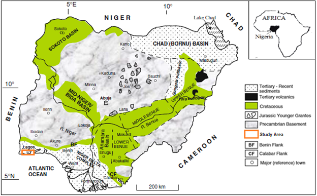
Figure 1: Generalized geological map showing the study area. Inset: Map of Africa showing Nigeria (modified from Obaje et al., 2011).
The litho-stratigraphy of the basin has been grouped into the following namely: The Abeokuta group (oldest), Ewekoro formation, Akinbo formation, Ososhun formation, Ilaro formation, coastal plain sands and Alluvium (recent) as shown in Table 1.
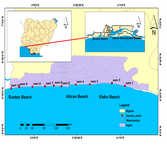
Figure 2: Sampling locations of Beach Sediments (Modified after Olanrewaju, 2018)
Sampling technique
Ten samples were randomly collected as surface samples from beaches in Lagos State (Atican Elegushi, Eleko and Suntan). All samples were collected from the beach front (beach surface). The importance of this sampling method was to cover a larger part of the study area. After removing the overburden, sampling was done at a distance of at least about 50m away from each station at a depth of 40cm. Global Positioning System (GPS) was employed to locate the precise geographical locations of sample points. At each station, beach sediment samples were collected using a hand auger and in some cases the builders’ trowel were used in order to obtain fresh representative samples. Each sample collected were bagged in nylons; labeled according to its locations and kept in the sample bag to avoid contamination of the sediments. On arrival at base, the samples were air dried and kept for subsequent analysis in the laboratory.
Heavy Metals Analysis
Eight heavy metals such as iron, lead, copper, nickel, cobalt, zinc, manganese and cadmium (Fe, Pb, Cu, Ni, Co, Zn, Mn and Cd) were analyzed using the Atomic Absorption Spectrophotometer. The samples were crushed into powder and 0.2g of the powdered samples were weighed into a beaker and were digested using the partial digested method using (Watts and Johnson, 2012) standard procedures. 10ml of Aqua Regia (which is an acid mixture of HCl and HNO3 in ratio 3:1 respectively). The mixture was heated up on hot plate or sand bath in a fume cupboard and heated to dryness. The procedure was repeated 4 times and heated to dryness. After heating, the elements that were attached to the surface of the crystal lattice dissociated from it. The diluted HCl was added to the caked sediment which stuck to the wall of the beaker in order to dissolve it. Little quantity of distilled water was also added to the mixture and filtered. The filtrate was analyzed with the Buck 210VGP Atomic Absorption Spectrophotometer (AAS), which analyses liquid minerals through partial digestion. The heavy metals were then analyzed and their concentrations recorded.
Distribution of Metals Concentration
The results of the geochemical analyses (Table 1) revealed that the Fe content is very high in all locations with values ranging from 4344.66 to 9154.86 ppm. The high concentration of Fe could be attributed to weathering and transportation of iron-bearing minerals such as micas and feldspars into the soils or sediments. Pb is relatively high in concentration in all locations with values from 133.39-778 ppm. Lead is considered to be a non-essential component for living organism species and is an accumulating poison. Therefore, it enters marine environment throughout the discharges (directly or from atmospheric removals) from the casting and sanitizing of lead; the burning of petroleum fuels containing lead parts and; to a smaller range, the melting of other metals. Ni concentration is very low in all locations with values ranging from 2.12-4.61 ppm. Nickel is a pervasive metal and takes place in soil, water, air, and in the atmosphere. The average content in the Earth's crust is about 0.008%. Levels in marine waters are found to be in the range of 0.2 and 0.7 μg/l (WHO, 1991). Nickel compounds are used as catalysts, pigments, and in batteries. Nickel from different industrial practices and other sources lastly reach to wastewater. Scums from wastewater treatment are dumped into ocean and land treatment (WHO, 1991). Dissolved nickel generally enters the marine environment through atmosphere depositions, urban runoff, industrial effluents, and municipal discharges and also from natural erosion of soils and rocks (Schultz, 2000).
Table 1. Geochemical results of the beach sediments (ppm)
|
Sample ID |
Fe |
Pb |
Ni |
Co |
Zn |
Mn |
Cu |
Cd |
|
L1 |
8979.20 |
778.08 |
3.75 |
0.001 |
17.89 |
42.97 |
21.35 |
0.001 |
|
L2 |
4344.66 |
345.91 |
3.01 |
0.001 |
12.24 |
38.32 |
43.38 |
0.001 |
|
L3 |
7901.4 |
418.12 |
3.41 |
0.001 |
14.46 |
43.38 |
19.42 |
0.001 |
|
L4 |
7029.24 |
418.12 |
3.1 |
0.001 |
18.45 |
41.44 |
16.74 |
0.001 |
|
L5 |
5057.74 |
379.43 |
3.58 |
0.001 |
18.79 |
54.02 |
18.24 |
0.001 |
|
L6 |
6274.78 |
133.39 |
2.58 |
0.001 |
16.68 |
43.93 |
19.42 |
0.001 |
|
L7 |
7568.14 |
191.31 |
2.78 |
0.001 |
10.69 |
44.53 |
22.86 |
0.001 |
|
L8 |
7999.26 |
161.65 |
2.12 |
0.001 |
11.13 |
56.29 |
18.03 |
0.001 |
|
L9 |
7568.14 |
273.92 |
3.12 |
0.001 |
13.46 |
68.48 |
18.67 |
0.001 |
|
L10 |
9154.86 |
183.16 |
4.61 |
0.001 |
12.3 |
56.55 |
19.7 |
0.001 |
|
MINIMUM |
4344.66 |
133.39 |
2.12 |
0.001 |
10.69 |
38.32 |
16.74 |
0.001 |
|
MAXIMUM |
9154.86 |
778.08 |
4.61 |
0.001 |
18.79 |
68.48 |
43.38 |
0.001 |
|
AVERAGE |
7187.742 |
328.309 |
3.206 |
0.001 |
14.609 |
48.991 |
21.781 |
0.001 |
According to Tebo et al. (1984) and Tebo (1998) cobalt has been commonly understood as a scavenged-type trace component in marine waters. Similar to iron, the slight solubility of cobalt while oxidizing to inorganic Co (III) appears preventing the accumulation in water column of the Pacific which is observing with nutrient-like trace components such as zinc. The oxidation of Co (II) to Co (III) can be done by co-precipitation with manganese oxides and by manganese-oxidizing microorganisms. The oxidation is understood to be a significant process for cobalt removal in the marine and coastal waters (Moffett and Ho, 1996). However, dust is considered to be a significant source of trace elements to the oceans, as estimated from the relative contribution of aeolian input to dissolved riverine input (Duce et al., 1991). The average concentration of cadmium in seawater have been assumed to be about 0.1μg/l or less (Yim, 1981). WHO, (1995) reported that current measurements of dissolved cadmium in surface waters of the open oceans gave values of < 5 ng/l. The vertical distribution of cadmium concentrations in marine waters is described by a surface depletion and shallow water supplementation, which relates to the form of nutrient concentrations in the considered areas (Shen and Boyle, 1987). Such distribution is considered to be the result of cadmium absorption by phytoplankton in surface waters and its transportation to the deep water, integration to organic fragments, and consequent releases. Zinc (Zn) concentration is low with values between 10.69 and 18.79 ppm. Zinc is one of the most abundant and mobile of the heavy metals and is transported in natural waters in both dissolved forms and attendant with suspended fragments (Mance and Yates, 1984). In seawater, considerably amount of zinc is found in dissolved form as inorganic and organic complexes. Conversely, zinc is a less toxic metal. Zinc is the most abundant trace element in the human body. Manganese (Mn) concentration in the sediment is a little higher than Cu with values ranging from 38.32 to 68.48 ppm. Manganese is an element that is naturally found in the tropical environment. It contains about 0.1% of the earth’s top layer as reported by NAS (1973) and found in rock, soil, water, as well as food. Hence, all humans are exposed to manganese, and it is a common element of the human body. Copper (Cu) concentration ranges from 18.03-21.35 ppm. The usages of copper include electrical cabling and plating, copper piping, photography, antifouling paints, formulation of pesticides and metals effluents from municipal wastes. The most industrial sources may include manufacturing, refining and coal-burning industries. These anthropogenic sources may lead to considerable concentrations entering the coastal and marine environments either directly through discharged sewage or industrial effluents or via depositions from the atmosphere (CCREM, 1987). It was reported that domestic sources are the main contributors of copper element in the ecosystems (Zaki, et al., 2012). Figure 3 and 4 are Bar charts of Fe and Pb distribution at the various locations; figure 5 shows the concentration of Ni, Zn, Mn and Cu at the sample locations.
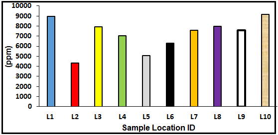
Figure 3. Distribution of Fe at the various sample locations.
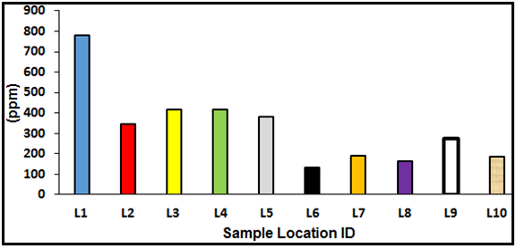
Figure 4. Variation in Pb concentrations at the sample locations.
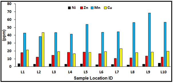
Figure 5. Ni, Zn, Mn and Cu concentrations at the sample locations.
Enrichment Factor
A standard approach to appraise the anthropogenic impact of heavy metal is to calculate the enrichment factor (EF) for metal concentrations above uncontaminated background levels (Fagbote and Olanipekun 2010). To identify anomalous metal concentration, geochemical normalization of heavy metal data to conservative elements, such as Al, Fe, and Si, has been employed. Several authors have successfully used Fe to normalize heavy metal contaminants (Muncha et al., 2003; Peres-Neto et al., 2006; Mediolla et al., 2008). In this study, the metals were normalized to Cd due to its mobility. According to Fagbote and Olanipekun (2010), the EF of a heavy metal in soil is defined as follows:
EF = [C-metal/C-normalizer]soil / [C-metal / C-normalizer] control……………(Eq.1)
where C-metal and C-normalizer are the concentrations of heavy metal and normalizer in soil and the control sample. Enrichment factor can be used to differentiate between the metals originating from anthropogenic activities and those from natural processes and to assess the degree of anthropogenic influence. The five contamination categories are recognized on the basis of the enrichment factor as follows (Sutherland, 2000): EF <2 is deficiency to minimal enrichment, EF = 2–5 is moderate enrichment, EF = 5–20 is significant enrichment, EF = 20–40 is very high enrichment, and EF >40 is extremely high enrichment. Enrichment factors are presented in Table 2. Cd was used as the normalizing element due to its least mobility. The Enrichment Factor of heavy metals around the ten locations shows that Cd (1.0) and Co (0.01) in all locations has no enrichment. Mn has minimal enrichment at locations 1,2,3,4 & 6, while it is moderately enriched in locations 5, 7, 8, 9 and 10 respectively (2.43, 2.00, 2.53, 3.08 and 2.55). Moderate enrichment was observed for Ni in all locations (2.03 – 4.41). Zn is significantly enriched in all locations (7.18 – 12.62). Fe is also significantly enriched in all location except location 2 and 5 having moderate enrichment (3.88 – 4.52). Cu is highly enriched (26.90 – 36.74) while extremely high enrichment factor was detected for Pb in all the locations (427.90 – 2059.62).
Table 2. Enrichment Factor of metals in the sediments (%)
|
Sample ID |
Fe |
Pb |
Ni |
Co |
Zn |
Mn |
Cu |
Cd |
|
L1 |
8.02 |
2059.62 |
3.59 |
0.01 |
12.02 |
1.93 |
34.31 |
1 |
|
L2 |
3.88 |
915.64 |
2.88 |
0.01 |
8.22 |
1.72 |
30.52 |
1 |
|
L3 |
7.06 |
1235.30 |
3.27 |
0.01 |
9.71 |
1.95 |
31.21 |
1 |
|
L4 |
6.28 |
1106.79 |
2.97 |
0.01 |
12.39 |
1.87 |
26.90 |
1 |
|
L5 |
4.52 |
1004.37 |
3.43 |
0.01 |
12.62 |
2.43 |
29.31 |
1 |
|
L6 |
5.60 |
1482.11 |
2.47 |
0.01 |
11.20 |
1.98 |
31.21 |
1 |
|
L7 |
6.76 |
506.41 |
2.66 |
0.01 |
7.18 |
2.00 |
36.74 |
1 |
|
L8 |
7.14 |
427.90 |
2.03 |
0.01 |
7.48 |
2.53 |
28.98 |
1 |
|
L9 |
6.76 |
725.08 |
2.99 |
0.01 |
9.04 |
3.08 |
30.01 |
1 |
|
L10 |
8.17 |
484.84 |
4.41 |
0.01 |
8.26 |
2.55 |
31.66 |
1 |
|
Average |
6.42 |
994.81 |
3.07 |
0.01 |
9.81 |
2.20 |
31.09 |
1 |
Assessment of Pollution Levels
Contamination Factor
The extent of contamination of sediment by a metal is often expressed mathematically in terms of a contamination factor calculated by:
CF= (Metal content) Sample / (Metal content) Background…………………..(Eq. 2)
Contamination of sediments could be from anthropogenic or geogenic sources, depending on the environment of deposition. However, a standard scheme for classifying the quality of sediments is presented in Table 3, while the contamination table of the beach sediments analyzed is shown in Table 4. The result revealed that all the sediments fell within low contamination factor and the value is CF<1 except Pb. This showed that the environment of deposition of the sediments is far from pollution sources.
Geo-accumulation Index
This has been used widely to evaluate the degree of metal contamination or pollution in terrestrial, aquatic, and marine environment Tijani and Onodera, (2009). The index of geo-accumulation (I-geo) of a metal in soil can be calculated using the formula previously applied by Asaah and Abimbola (2005) and Mediolla et al. (2008) as shown below:
Igeo = log2 (Cn / 1.5 Bn) ………………………………………………………(Eq. 3)
Where Cn is the measure of concentration of the examined metal in the soil and Bn is the geochemical background concentration of the same metal. The factor of 1.5 is introduced to minimize the effect of possible variations in the background or control values which may be attributed to lithogenic variations in the sediment (Mediolla et al., 2008).
Table 3. Standard contamination scheme for sediments (Hakanson, 1980)
|
CF Value |
Class |
Quality of sediment |
|
CF<1 |
1 |
Low contamination factor |
|
1 ≤ CF |
2 |
Moderate contamination factor |
|
3 ≤ CF<6 |
3 |
Considerable contamination factor |
|
CF ≥ 6 |
4 |
Very high contamination factor |
Degree of Contamination (Cd), Modified Degree of Contamination (mCd), Pollution Load Index (PLI)
The degree of contamination (Cd) is the sum of individual contamination factor of the pollutant (Hakanson, 1980). This parameter is aimed at providing a measure of the degree of overall contamination in surface layers in particular sampling site. The degree of contamination (Cd) is calculated by the equation (Hakanson, 1980):
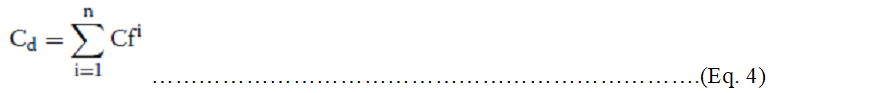
Table 4. Contamination Factors
|
Sample ID |
Fe |
Pb |
Ni |
Co |
Zn |
Mn |
Cu |
Cd |
|
L1 |
0.178 |
45.769 |
0.079 |
0.0001 |
0.267 |
0.043 |
0.763 |
0.022 |
|
L2 |
0.086 |
20.877 |
0.064 |
0.0001 |
0.183 |
0.038 |
0.678 |
0.022 |
|
L3 |
0.157 |
27.451 |
0.073 |
0.0001 |
0.216 |
0.043 |
0.694 |
0.022 |
|
L4 |
0.139 |
24.588 |
0.066 |
0.0001 |
0.275 |
0.041 |
0.598 |
0.022 |
|
L5 |
0.1 |
22.294 |
0.076 |
0.0001 |
0.28 |
0.054 |
0.651 |
0.022 |
|
L6 |
0.125 |
7.846 |
0.055 |
0.0001 |
0.249 |
0.044 |
0.694 |
0.022 |
|
L7 |
0.15 |
11.253 |
0.059 |
0.0001 |
0.159 |
0.045 |
0.816 |
0.022 |
|
L8 |
0.159 |
9.509 |
0.045 |
0.0001 |
0.166 |
0.056 |
0.644 |
0.022 |
|
L9 |
0.15 |
16.113 |
0.066 |
0.0001 |
0.201 |
0.068 |
0.667 |
0.022 |
|
L10 |
0.182 |
10.774 |
0.098 |
0.0001 |
0.184 |
0.057 |
0.704 |
0.022 |
|
Average |
0.14 |
19.65 |
0.07 |
0.0001 |
0.22 |
0.05 |
0.69 |
0.02 |
The degree of metal pollution is assessed in terms of seven contamination classes based on the increasing numerical value of the index as follows: Huu et al., (2010).; I-geo<0 means unpolluted, 0≤I-geo<1 means unpolluted to moderately polluted, 1≤I-geo<2 means moderately polluted, 2≤I-geo<3 means moderately to strongly polluted, 3≤I-geo<4 means strongly polluted, 4≤I-geo<5 means strongly to very strongly polluted and I-geo≥5 means very strongly polluted. The negative values in Fe, Ni, Co, Zn, Mn, Cu and Cd indices of geo-accumulation are as a result of no pollution (Table 5). Pb is moderately to strongly polluted in locations 6 & 10 (2.387 – 2.9), strongly polluted in locations 2, 5 & 9 (3.42 – 3.8), strongly to very strongly polluted in locations 1,3 & 4 (4.0 – 4.9).
Table 5. Geo-accumulation index for the heavy metals in the sediments
|
Sample ID |
Fe |
Pb |
Ni |
Co |
Zn |
Mn |
Cu |
Cd |
|
L1 |
-3.07 |
4.93 |
-4.23 |
-13.66 |
-2.49 |
-5.13 |
-0.98 |
-6.08 |
|
L2 |
-4.12 |
3.76 |
-4.55 |
-13.66 |
-3.04 |
-5.29 |
-1.15 |
-6.08 |
|
L3 |
-3.26 |
4.19 |
-4.37 |
-13.66 |
-2.80 |
-5.11 |
-1.11 |
-6.08 |
|
L4 |
-3.43 |
4.04 |
-4.51 |
-13.66 |
-2.45 |
-5.18 |
-1.33 |
-6.08 |
|
L5 |
-3.90 |
3.90 |
-4.30 |
-13.66 |
-2.42 |
-4.80 |
-1.20 |
-6.08 |
|
L6 |
-3.59 |
2.39 |
-4.77 |
-13.66 |
-2.59 |
-5.09 |
-1.11 |
-6.08 |
|
L7 |
-3.32 |
2.91 |
-4.66 |
-13.66 |
-3.23 |
-5.07 |
-0.88 |
-6.08 |
|
L8 |
-3.24 |
2.66 |
-5.06 |
-13.66 |
-3.18 |
-4.74 |
-1.22 |
-6.08 |
|
L9 |
-3.32 |
3.43 |
-4.50 |
-13.66 |
-2.90 |
-4.45 |
-1.17 |
-6.08 |
|
L10 |
-3.05 |
2.85 |
-4.08 |
-13.66 |
-3.03 |
-4.73 |
-1.09 |
-6.08 |
|
Average |
-3.43 |
3.50 |
-4.50 |
-13.66 |
-2.81 |
-4.96 |
-1.12 |
-6.08 |
where Cf is the contamination factor of each element; n is the number of elements under investigation. A modified form of the Hakanson (1980) equation proposed by Abrahim and Parker (2008) for the calculation of the overall degree of contamination was used in this paper and determined by the equation:

where, mCd is modified degree of contamination, n is the number of analyzed element and Cfi is the contamination factor; the Cd and mCd data for this work are presented in Table 6. Abrahim and Parker (2008) proposed the following classes for the modified degree of contamination: mCd< 1.5, nil to very low degree of contamination; 1.5 ≤ mCd< 2, low degree of contamination; 2 ≤ mCd< 4, moderate degree of contamination; 4 ≤ mCd< 8, high degree of contamination; 8 ≤ mCd< 16, very high degree of contamination; 16 ≤ mCd< 32, extremely high degree of contamination and mCd ≥ 32 means ultra-high degree of contamination. Results from this analysis classified the sample sites as having moderate degree of contamination.
Table 6: Degree of Contamination (Cd), Modified Degree of Contamination (mCd) Pollution Load Index (PLI) of the heavy metals in the beach sediments.
|
Sample ID |
Degree of contamination |
Modified degree of contamination |
Pollution Load Index |
|
L1 |
48.12 |
6.02 |
0.10 |
|
L2 |
23.95 |
2.99 |
0.08 |
|
L3 |
31.66 |
3.96 |
0.09 |
|
L4 |
29.73 |
3.72 |
0.09 |
|
L5 |
28.48 |
3.56 |
0.09 |
|
L6 |
15.04 |
1.88 |
0.07 |
|
L7 |
19.50 |
2.44 |
0.08 |
|
L8 |
18.60 |
2.33 |
0.07 |
|
L9 |
26.29 |
3.29 |
0.09 |
|
L10 |
22.02 |
2.75 |
0.09 |
|
AVERAGE |
26.34 |
3.3 |
0.08 |
|
MAX |
48.12 |
6.0 |
0.10 |
|
MIN |
15.04 |
1.9 |
0.07 |
The Pollution Load Index (PLI) was developed by Tomlinson et al. (1980) to compare pollution levels between sites and propose a necessary line of action. The PLI was computed based on the method proposed by Tomlinson et al. (1980). The PLI of the area was evaluated by obtaining the n-root from the n-CFs that were obtained for all the elements. This parameter is expressed as:
PLI = (Cf1 × Cf2 × Cf3 ×..........Cfn)1/n
Where n is the number of elements and Cf is the contamination factor, the PLI values are shown in Table 6. According Tomlinson et al. (1980), a Pollution Load Index (PLI) <1 denote perfection; PLI = 1 present that only baseline levels of pollutants are present and PLI > 1 would indicate deterioration of site quality. The results gotten indicates that the PLI values are less than 1, which denotes perfection. Likuku et al. (2013) proposed that a PLI value of ≥1 indicates an immediate intervention to ameliorate pollution; 0.5 ≤ PLI < 1 suggests that more detailed study is needed to monitor the site, whilst a value of < 0.5 indicates that there is no need for drastic rectification measures to be taken. All the PLI values are less than 0.5, implying that there is no need for drastic rectification measures to be taken
Potential Ecological Risk Index
The ecological risk index (Eri) evaluates the toxicity of trace elements in sediments. Environments contaminated by heavy metals can cause serious ecological risks and negatively impact human health due to various forms of interaction. Hakanson (1980), proposed a method for the potential ecological risk index (RI) to assess the characteristics and environmental behavior of heavy metal contaminants in sediments. To calculate the Eri for individual metals, we used the expression (4):
Eri = Tri * Cfi …………………………………………………………….(Eq. 6)
where Cfi is the contamination factor and Tr is the toxicity coefficient of each metal whose standard values are Cd = 30, Co = 5, Cu = 5, Ni = 5, Pb = 5, Cr = 2, Mn = 1, and Zn = 1 (Hakanson, 1980); Xu, 2008). To calculate the potential response rate to the toxicity of all the studied heavy metals (RI), the equation below is used:

According to Hakanson (1980), the following terminologies are suggested for the Er and RI values: (i) Er <40, low ecological risk; 40 < Er ≤80, moderate ecological risk; 80 < Er ≤160, appreciable ecological risk; 160 < Er ≤320, high ecological risk; and >320, serious ecological risk; (ii) RI <150, low ecological risk; 150 < RI <300, moderate ecological risk; 300 < RI <600, high ecological risk; and RI ≥ 600, significantly high ecological risk. Ni, Co, Zn, Mn, Cu and Cd showed low ecological risk at all the locations except for Pb that showed moderate ecological risk.
Table 7. Evaluation on potential risk of heavy metals pollution in sediments from
|
Sample ID |
Ecological Risk Index (Eri) |
(RI) |
Risk grade |
||||||
|
Pb |
Ni |
Co |
Zn |
Mn |
Cu |
Cd |
|||
|
L1 |
228.85 |
0.395 |
0.0005 |
0.267 |
0.043 |
3.815 |
0.66 |
234.03 |
Moderate |
|
L2 |
104.39 |
0.32 |
0.0005 |
0.183 |
0.038 |
3.39 |
0.66 |
108.98 |
Low |
|
L3 |
137.26 |
0.365 |
0.0005 |
0.216 |
0.043 |
3.47 |
0.66 |
142.01 |
Low |
|
L4 |
122.94 |
0.33 |
0.0005 |
0.275 |
0.041 |
2.99 |
0.66 |
127.24 |
Low |
|
L5 |
111.47 |
0.38 |
0.0005 |
0.28 |
0.054 |
3.255 |
0.66 |
116.1 |
Low |
|
L6 |
39.23 |
0.275 |
0.0005 |
0.249 |
0.044 |
3.47 |
0.66 |
43.93 |
Low |
|
L7 |
56.27 |
0.295 |
0.0005 |
0.159 |
0.045 |
4.08 |
0.66 |
61.5 |
Low |
|
L8 |
47.55 |
0.225 |
0.0005 |
0.166 |
0.056 |
3.22 |
0.66 |
51.87 |
Low |
|
L9 |
80.57 |
0.33 |
0.0005 |
0.201 |
0.068 |
3.335 |
0.66 |
85.16 |
Low |
|
L10 |
53.87 |
0.49 |
0.0005 |
0.184 |
0.057 |
3.52 |
0.66 |
58.78 |
Low |
|
AVERAGE |
98.24 |
0.34 |
0.0005 |
0.22 |
0.05 |
3.45 |
0.66 |
102.96 |
Low |
Potential Contamination Index (Cp)
The potential contamination index can be calculated by the following method:
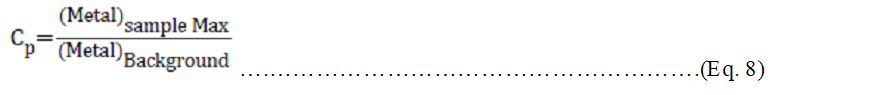
Where (Metal) sample Max is the maximum concentration of a metal in sediment, and (Metal) Background is the average value of the same metal in a background level. Cp values were interpreted as proposed by Dauvalter and Rognerud (2001) where Cp<1 indicates low contamination; 1<Cp<3 is moderate contamination; and Cp>3 is severe contamination. All the metals have Cp values less than 1, except Lead (Pb) with a value of 39.
Interrelationships among Heavy Metals
Correlation coefficients reveal the interrelationships between elements. However, the correlation analysis of elements shows a positive correlation between Iron Fe & Pb. Ni, Mn, Cu and Cd with the following coefficients such as Fe-Pb (0.152) Fe-Ni (0.326), Fe-Mn (0.280), Fe-Cu (0.332), Fe-Cd (0.177). Pb is positively correlated with Ni; Pb-Ni (0.366), with Zn; Pb-Zn (0.566) and with Cu; Pb-Cu (0.107). Ni correlates positively with Zn; Ni-Zn (0.228), with Manganese; Ni-Mn (0.110) and with copper; Ni-Cu (0.138). However, Zn correlates negatively with Manganese; Zn-Mn (-0.227), with copper; Zn-Cu (-0.337) and with Cadmium; Zn-Cd (-0.077) and Mn correlates positively with Cd; Mn-Cd (0.467). This revealed that elements with positive correlation are abundant in the geochemical system while those with negative correlation are depleted (Table 8).
Table 8. Correlation showing interrelationship of the heavy metals in the sediments
|
|
Fe |
Pb |
Ni |
Co |
Zn |
Mn |
Cu |
Cd |
|
Fe |
1 |
|
|
|
|
|
|
|
|
Pb |
0.152 |
1 |
|
|
|
|
|
|
|
Ni |
0.326 |
0.366 |
1 |
|
|
|
|
|
|
Co |
-0.402 |
-0.803 |
-0.278 |
1 |
|
|
|
|
|
Zn |
-0.187 |
0.566 |
0.228 |
-0.371 |
1 |
|
|
|
|
Mn |
0.28 |
-0.356 |
0.11 |
0.224 |
-0.227 |
1 |
|
|
|
Cu |
0.332 |
0.107 |
0.138 |
-0.409 |
-0.337 |
-0.207 |
1 |
|
|
Cd |
0.177 |
-0.62 |
-0.133 |
0.667 |
-0.077 |
0.467 |
-0.253 |
1 |
Descriptive Statistical Analysis
Pb which is the most enriched metal in the sediments is positively skewed and it has a mean value of 7187.742, Pb has a mean value of 333.164, Ni has a mean value of 3.206, Co has a mean value of 0.002, Zn has a mean value of 3.1097, Mn has mean value of 9.41922, Cu has a mean value of 1.72660. Iron is negatively skewed (Table 9). However, the coefficient of variance revealed the dominance of heavy metals such Fe, Pb, Mn and Cd in the system while Ni & Co are in minor quantities (Table 9). The high levels of Pb observed is as a result of anthropogenic impact, which is chiefly of environmental pollution which could probably be associated with activities such as sewage, cement bags washing, domestic and industrial wastes that took place within and around the lagoon and environs.
Table 9. Descriptive statistics for the beach sediment samples
|
Metals in ppm |
Min. |
Max. |
Mean |
Standard deviation |
Coefficient of variance (r) |
Skewness |
Kurtosis |
|
Fe |
4344.660 |
9154.860 |
7187.742 |
1563.997 |
2446088.417 |
-0.691 |
-0.231 |
|
Pb |
133.390 |
778.080 |
333.164 |
194.580 |
37861.660 |
1.352 |
2.198 |
|
Ni |
2.12 |
4.61 |
3.206 |
0.68787 |
.473 |
0.587 |
1.094 |
|
Co |
0.002 |
0.002 |
0.002 |
0.0000 |
.000 |
|
|
|
Zn |
10.69 |
18.79 |
14.6090 |
3.10977 |
9.671 |
0.206 |
-1.769 |
|
Mn |
38.32 |
68.45 |
48.988 |
9.41922 |
88.722 |
1.008 |
0.368 |
|
Cu |
16.74 |
22.86 |
19.3420 |
1.72660 |
2.981 |
0.813 |
1.062 |
|
Cd |
0.002 |
0.002 |
0.00 |
0.0000 |
2446088.417 |
|
|
The result of the geochemical analysis has presented an increasing order of the heavy metals concentration in the sediments to reflect the sequence as follows; Fe>Pb>Mn>Cu>Zn>Ni>Co=Cd. By normalizing the metals detected, Cadmium (Cd) was used to calculate the Enrichment Factor and Geo-accumulation Index due to its mobility. Results revealed high levels of Fe and Pb enrichment in the sediments which were linked with the deleterious effect of anthropogenic activities on the Lagos beaches such as dumping and biodegradation of wastes, industrial effluents etc. The results revealed that the contamination levels is within high to very high contamination which can also be linked to increased human activities on the beaches such as indiscriminate sewage disposal or activities of some white garment churches or fun seekers . Based on this study, the framework for mandatory action should be initiated for regular assessment of Lagos lagoon to ensure conservation of Lagos lagoon coastal resources. There should be strict regulations to control the dumping of chemical contaminants into the lagoon with enforcement of penalties imposed on defaulters. Enlightenment programs for the public on their mode of disposing waste water and other harmful substances into drainages. Also, the high level of Pb concentrations in the sediments poses a high level of risk in siting boreholes and hand dug wells at or close to the studied area as these could lead to serious health challenges and disastrous consequences.
I hereby acknowledge Olarenwaju Adeyemi Ejuwa and Oluwatobi Ife Omoniyi who served as my technical partners and field assistants for their tremendous efforts during field work and data gathering for the sucessful completion of this research. I am very grateful for all your efforts.
Abrahim, G.M.S., and Parker, R.J. (2008). Assessment of heavy metal enrichment factors and the degree of contamination in marine sediments from Tamaki Estuary, Auckland, New Zealand. Environ. Monitoring and Assessment. 136: 227–238. PMid:17370131
View Article PubMed/NCBIAdeyemo, O. K., Adedokun, O. A., Yusuf, R. K., Adeleye, E. A. (2008). Seasonaal changes in physio-chemical parameters and nutrient load of river sediment in Ibadan city, Nigeria. Global Nest Journal 10(3): 326 – 336.
Asaah A.V. and Abimbola A.F. (2005). Heavy metal concentrations and distribution in surface soils of the Bassa Industrial Zone 1 Doula, Cameroon. The Journal for science and Engineering 31(2A): 147-158.
CCREM, (1987). Canadian water quality guidelines. Prepared by the task force on Water Quality Guidelines.
Dauvalter, V. and Rognerud, S. (2001). Heavy metal pollution in sediments of the Pasvik River drainage. Chemosphere 42: 9-18. 00094-1
View ArticleFagbote, E. O., Olanipekun, E. O., (2010): Evaluation of the status of heavy metal pollution of sediment of Agbabu Bitumen Deposit Area, Nigeria. European Journal of Science Research, 41:373–382
Hakanson, L. (1980). An Ecological Risk Index for Aquatic Pollution Control, a Sedimentological Approach. Water Resources, 14:975-1001.
Huu, H.H., Rudy, S. and Van Damme (2010). Distribution and contamination status of heavy metals in estuarine sediments near Cau ong harbor, Ha long Bay, Vietnam. Geology Belgica 13 (1-2): 37-47.
Iwugo, O.K.O., D'arcy B., Andoh, R. (2003): Aspects of Land-based pollution of an African Coastal Megacity of Lagos.Proceedings of the International Specialised IWA Conference, Dublin, Ireland.
Mance, G. and Yates, J. (1984). Proposed Environmental Quality Standards for List III----organisms, Ocassional Publication No.2 In: T.R Crompton, Marine Biology Association, Plymouth, USA, 495p. PMid:6748931
PubMed/NCBIMediolla, L.L., Domingues, M.C.D. and Sandoval M.R.G. (2008). Environmental Assessment of and Active Tailings Pile in the state of Mexico (Central Mexico). Research Journal of Environmental Sciences. 2(3): 197-208.
View ArticleMoffett, J.W. and Ho, J. (1996). Oxidation of cobalt and manganese in seawater via a common microbially catalyzed pathway. Geochimica et Cosmochimica Acta 60(18):3415-3424. 00176-7
View ArticleMuncha, A.P., Teresa, M., Vasconcelos, S.D., Adriano, B. (2003). Macrobenthic Community in the Douro Estuary: Relations with Trace metals and Natural sediment characteristics. Environmental Pollution, 121(2): 169-80. 00229-4
View ArticleNAS (1973): Medical and biological effects of environmental pollutants: manganese. Washington, DC, National Academy of Science, National Academy Press.
Obaje, N. G., Musa, M. K. Odoma, A. N. and Hamza, H. (2011). The Bida Basin in north-central Nigeria: sedimentology and petroleum geology. Journal of Petroleum and Gas Exploration Research, 1(1), 001-013
Olanrewaju, A.E. (2018). Sedimentological Studies of the Beach Sediments in Lagos State, Southwestern Nigeria. Federal University of Technology, Akure, B.Sc Thesis (published), 76p.
Omatsola, M.E. and Adegoke, S.O. (1981). Tectonic evolution and Cretaceous Stratigraphy of the Dahomey Basin Journal of. Mining Geology, 18(1): 130- 136.
Prasanth, K., Sreekala, P., Sandeep, S., Kripa, P., Sreejesh, K. (2013): Heavy Metals and its Fractions in Soils of Koratty Region, Kerala. Research Journal of Recent Sciences 2277- 2502.
Peres-Neto, P.R., Legendre, P., Dray, S., Borcard, D. (2006). Variation portioning of species data matrix estimation and comparison of fractions. Ecology, 87(10): 2614-2625 87[2614:VPOSDM]2.0.CO;2
View ArticlePuttaiah, E.T., Kiran, B.R., (2007). Heavy metal transport in a sewage fed lake of Karnataka, India. Proceedings of Taal. The 12th world lake conference. 347-354.
Saroja, K. Barik, Pradipta, R. Muduli, Bita Mohanty, Prasanta Rath, Srikanta Samanta (2018). Spatial distribution and potential biological risk of some metals in relation to granulometric content in core sediments from Chilika Lake, India. Environmental Science and Pollution Research (Springer), 1:572-587
Shen, T.G., Boyle, E.A. (1987). Lead in Corals: Reconstruction of historical industrial fluxes to the surface ocean. Earth & Planetary Science letters, 82(3):289-304. 90203-2
View ArticleSchultz, W. (2000). Multiple reward signals in the brain. Neuroscience, 1(3):199-207. PMid:11257908
PubMed/NCBISuciu, I., Cosma, C., Todika, M., Bolboaca, S. D., Jantschi, L. (2008): Analysis of soil heavy metal pollution and patern in central Transylvanian. International. Journal of. Molecular Science, 9: 434 – 453
View ArticleSutherland, R.A. (2000). Bed sediment-associated trace metals in an urban stream. Oahu, Hawaii. Environmental Geology 39: 611-37.
View ArticleTijani, M.N., Onodera, S., (2001). Hydrogeochemical Assessment of Metal Contamination in an Urban Drainage System. A case study of Osogbo Township, Southwestern Nigeria. Journal of Water Resource & Protection, 1(3):1-10.
Tebo, B.M. (1998). Comment on the comment by A.W.M.G Souren on "Oxidation of Cobalt and Manganese in sea water via a-common microbially catalyzed pathway. Geochim, Cosmochim. Act. 62:357-358.
Tebo, B.M., Kenneth, H.N., Emerson, S., Jacobs, L. (1984). Microbial mediation of Mn (II) and Co (II) precipitation at the O2/H2S interfaces in two anoxic fjords. Limnol Oceanage, 29(6):1247-1258.
View ArticleThakur, A.K., Ojha, C.S.P., Grischek, T., Ray, C. Saandhu C. (2010). Water Quality Improvement through river bank filteration in extreme environmental conditions. Journal of Indian Water Works Association, 43(2): 106-115.
Tomlinson D.L., Wilson J.G., Harris C.R., and Jeffney D.W. (1980). Problems in the Assessment of Heavy Metal Levels in Estuaries and the Formation of a Pollution Index, Helgol. Wiss. Meeresunters, Vol. 33, pp 566-572.
View ArticleTrenhaile, A.S., (1997). Coastal Dynamics and Landforms, Oxford University Press
Watts, D.W. and Johnson, M.H. (2012). Geochemical mapping using stream sediments inwest-central Nigeria. Implications for environmental studies and mineral exploration in west Africa. Applied geochemistry, 27 (6): 1035-1062.
View ArticleWHO (1991). Environmental Health Criteria 124, LINDANE, World Health Organization A report published jointly by the United Nations Environment Program, the International Labor Organization and the World Health Organization, Genevea, 214p.
WHO (1995). World health report: Summary; provisional agenda item 10. 16p, Mondiale de la santé.
Yim, Wyss W.S. (1981). A comparative Evaluation of Oysters, muscles and sediments as indicators of Trace metal in Hong Kong Waters. Marine Ecology Progress Series, 6(3)285-293.
Zaki, M.A., Labib, E.M., Nour, A.M, Tonsy, H.D., Mahmoud, S.H., (2012). Some medicinal plants diet on mono sex Nile Tilapia (Oreochromis niloticus), growth, performance, feed utilization and physiological parameters. APCBEE Procedia, 4:220-22
View Article