Konstantinos Ath. Konstantopoulos,
Email: kkonstantopoulos@eap.gr
© 2019 Sift Desk Journals. All Rights Reserved
VOLUME: 3 ISSUE: 2
Page No: 386-394
Konstantinos Ath. Konstantopoulos,
Email: kkonstantopoulos@eap.gr
Konstantinos Ath. Konstantopoulos1, George Ch. Miliaresis 2
1. Hellenic Open University, School of Science & Technology, Address: 4 Tzortz Street, P.C. 106 77, Kaniggos Square, Athens, Greece
Email: kkonstantopoulos@eap.gr ; Tel: +30 210 9097206, Fax: +30 210 9097201
2. Open University of Cyprus, Environmental Protection & Management, Adress: 38, Tripoleos Str., Athens, 104-42, Greece.
Email: miliaresis.g@gmail.com, george.miliaresis@ouc.ac.cy ; Tel: +30-6971.633.732, Fax: +30-210-5128712
Chenghao Wang(cwang210@asu.edu)
Konstantinos Konstantopoulos, Unsupervised landslide risk dependent terrain segmentation on the basis of historical landslide data and geomorphometrical indicators.(2018)SDRP Journal of Earth Sciences & Environmental Studies 3(2)
The terrain segmentation to zones of high to low landslide risk is key issue in urban and technical works planning in western Greece where landslide hazard is a key factor in loss of properties while significant damages to road network take place. The study area includes the prefecture authority of Achaia where landslide hazard is amplified by the lithology (flysch and alluvial deposits), fracture systems, down-cutting erosion, severe rainfalls, and earthquakes. The landslide database of the Institute for Geology and Mineral Exploration of Greece is used to derive the occurrence of landslides within the study area. Totally 82 sites of landslide occurrence were considered within the study area. The innovative idea in this research effort is to use terrain attributes: (a) That apply to each grid point of a digital elevation model and (b) They refer to an extended neighbor that is relevant to each grid point under consideration. So in this approach an extended neighbor that varies per grid point per terrain attribute as well as shape terrain attributes are used to characterize the geomorphometry of the study area. Under a trial and error procedure 13 terrain attributes (Channel Network Distance, Profile Curvature, Length Slope Factor, Valley Depth, Downslope Curvature, Convergence Index, Flow Path Length, Plan Curvature, Positive Openness, Topo Wetness Index, Total Catchment Area, Mass Balance Index, Upslope Curvature) presenting the minimum correlation between them were selected. K-means clustering defined 8 terrain classes. Each terrain class is represented by the centroid vector and its spatial extent. The percent landslide occurrence within the percent area occupied by each terrain class, is used to define a new landslide susceptibility index that is useful for hazard/risk assessment, land use and land cover studies as well as rural and urban planning within the study area.
Keywords: landslides, digital elevation model, geomorphometrical characterization, urban planning.
Landslides are destructive geological processes which cause enormous damage to human settlements, roads as well as to the infrastructure related to the management and exploitation of natural resources (Pandey 1987). Landslides are the result of complex interaction among geologic, geomorphologic and meteorologic factors (Gao et al. 2015). Spatial data related to these factors can be derived by remote sensing techniques and ground based information while historical information captures the frequency of landslides events (Sangar and Kanungo 2004). For non-damaging natural terrain landslides, the location of their occurrence must be close to human activities, to catch the attention otherwise will not be reported (Dai and Lee, 2002). This causes a major drawback in the estimation of landslide risk in natural terrain (areas covered by natural vegetation-forests, non cultivated, non urban, non rural lands) on the basis of historic records (Gao et al. 2015).
Nowadays, remote sensing data and image processing were used to the mapping of landslides and the determination of temporal associations between land-sliding events and surface conditions (Sangar and Kanungo 2004) while assessment of landslide susceptibility has been attempted in a wide variety of geographic information systems using diverse approaches (Costanzo et al. 2014). These methods are based on the integration of combined effect of the spatial factors identified to be important in assessing slope instability. In these approaches, the spatial factors where integrated on an artificial regular-grid terrain-partition scheme (Shirzadi et al. 2017) that was not related to the geomorphologic entities that occur in the natural terrain.
At the same time various digital image processing and G.I.S. techniques are being developed in order to automate the qualitative interpretation of geomorphologic features (Miliaresis et al. 2005). These methods allow terrain segmentation to elementary geomorphic objects and subsequent parametrically representation of objects on the basis their spatial 3-dimensional arrangement. The use of these techniques is stimulated by the availability of the global coverage SRTM moderate resolution elevation data (Miliaresis and Paraschou 2005) that is freely available through the internet (SRTM DEM, 2017).
In the previous approaches, terrain segmentation was based on a regular grid, the most critical effect being the grid resolution (Dhakal et al. 2000). For example, a regular grid partition framework could be composed of cells with size 20 times the DEM spacing. Thus each cell would be composed from 400 DEM points. Then, raster maps are created for each spatial (hydrology, vegetation, climate, geology, geomorphology, etc.) factor (Chau et al. 2004). In each cell, a value quantifies the spatial factor magnitude. Thus, a major drawback is involved in the subsequent raster maps combination since values are related not to geomorphologic entities but to an artificial regular grid partition scheme.
The innovative idea in this research effort is to use terrain attributes: (a) that apply to each grid point of a digital elevation model and (b) they refer to an extended neighbour that is relevant to each grid point under consideration. So in this approach an extended neighbour that varies per grid point per terrain attribute is used to characterize the geomorphometry (Pike et al 2008) of the study area. In the proposed approach the landslide occurrence will be related to the intensity of flow, transportation and erosion phenomena, as well as terrain shape, derived from an extended neighbour in relation to the static pixel based approaches.
First the study area and the data are introduced. Then landslide inventory analysis, knowledge conceptualization and statistical analysis identified the geomorphometric attributes. Then a methodology is developed that segments the terrain to terrain classes will landslide occurence is used to determine the landslide risk per terrain class within the study area.
STUDY AREA
The study area is enclosed by the following rectilinear co-ordinates minimum X=266,088 m, maximum X=358,488 m, minimum Y=4,182,424 m and maximum Y=4,248,199 m, based on the Greek Geodetic Reference System of 1987 (Mugnier 2002). It coincides with Achaia prefecture in the Western Greece (Figure 1).
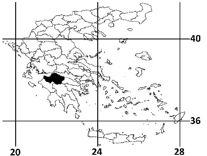
Figure 1. The study area (black polygon the coincides to Achaia prefecture) within a latitude, longitude (in degrees) map of Greece that depicts the borderlines of the prefecture authorities.
The geological setting and tectonics of western Greece is summarized by Miliaresis et al. (2005) as follows. The formations consisting the geological basement are limestone, dolomites and dolomitic limestones, schists and cherts, and flysch. Intense and multifarious fracturing is evident and calcareous rocks are also karstic. Flysch mainly consists of marls, sandstones, siltstones. The post-alpine sediments are represented by the Neogene and Quaternary deposits. Synclinal and anticlinal folds of extensive length and with an axis directed N-S are intersected by two main fault systems in the NW-SE and NE-SW directions. In southern part the faults are in N-S and E-W directions while thrusts are generally directed N-S. The tectonic picture is completed by the post-alpine gravity faults.
LANDSLIDE INVENTORY
The landslides in Western and Central Greece occur basically in the flysch, the neogene, the upthrusts formations and the loose quaternary deposits (Miliaresis et al 2005). The landslide data of the geo-database of ground failures of Institute for Geology and Mineral Exploration (IGME) of Greece (NGGF 2018; Poyiadji 2007) was used for risk analysis. The spatial distribution of landslides within the study area is depicted in Figure 2. Landslides were reported in the mountainous terrain, along settlements, and parallel to the coast along the Athens-Patras national highway (Miliaresis et al 2005).
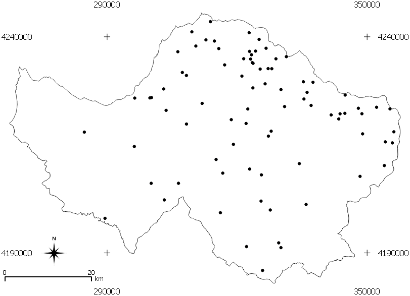
Figure 2. The landslide occurrence within the study area (projected the to Greek Geodetic Reference system of 1987).
It should be noted that the most landslides records are either failures of man-made or natural terrain landslides that lead to death, injury, or interruption of human activities. For non-damaging natural terrain landslides, the location of their occurrence must be close to human activities, to catch the attention otherwise will not be reported (Miliaresis et al. 2005). Although it is very unlikely that the data compiled are complete, the data set is considered reliable and constitutes a good basis for landslide risk analysis.
ELEVATION DATA
NASA collected elevation data for much of the world using a radar instrument aboard the space shuttle that orbited the earth from the 11th through the 22nd of February 2000 (Farr and Kobrick 2000). The space shuttle topography mission (SRTM) digital elevation model (DEM) is projected to a latitude/longitude grid referenced to WGS-84 (horizontal datum) while elevations are referenced to EGM96 geoid (vertical datum). The DEM data is available to 1, 3 and 30 arc seconds spatial resolutions.
In this study the 3 arc seconds SRTM DEM was used with spacing approximately 92.6 m at the equator (Miliaresis and Paraschou 2005). The DEM data was reprojected to the Greek Geodetic Reference system of 1987 (Mugnier 2002) and resampled by nearest neighbor at 100 m grid spacing. It contains 901 columns and 626 rows. The elevation is within the interval 0 to 2,096 m ( Figure 3). The accuracy of the DEM data together with the data spacing adequately supports computer applications that analyze hypsographic features to a level of detail similar to manual interpretations of information as printed at map scales not larger than 1:50,000 (Miliaresis and Paraschou 2005).
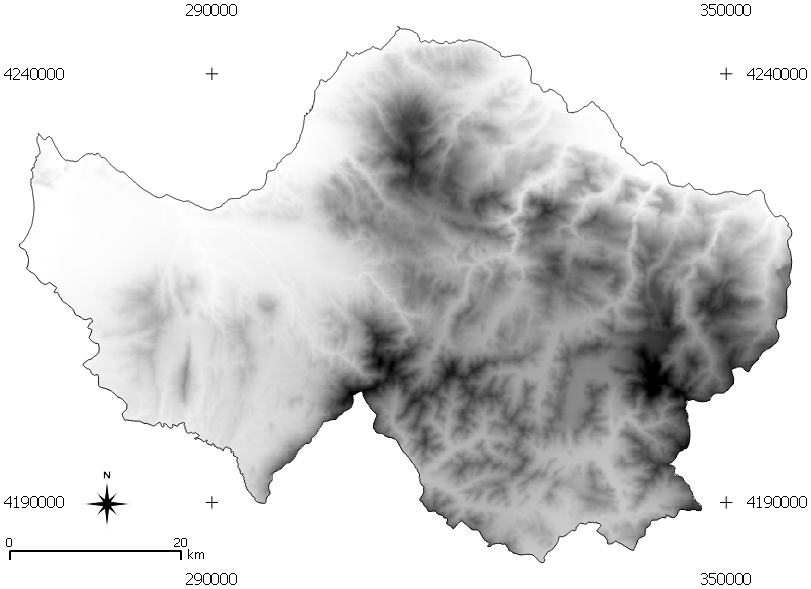
Figure 3. The DEM of the study area (the darker a pixel, the greater it’s elevation).
TERRAIN ATTRIBUTES
In the current approach an extended neighbor that varies per grid point per terrain attribute as well as shape terrain attributes are used to characterize the geomorphometry of the study area. So the landslide occurrence will be related to the intensity of flow, transportation and erosion phenomena, as well as terrain shape (Pike at al 2008), derived from an extended neighbour (that is relevant to each grid point under consideration) in contrast to the static pixel based approaches that considers the geomorphometric properties within a fixed size kernel. Various terrain attributes are tested. The selection criterion considers the terrain attributes with minimum absolute correlation (Landam and Everitt 2004) in between them (Table 1).
Table 1. Cross correlation of terrain attributes.
|
Cross Correlation |
CC |
CND |
ProfC |
Lsf |
VD |
DC |
CI |
FPL |
PlanC |
PO |
TWI |
TCA |
MBI |
UC |
|
Channel network distance |
CND |
1 |
0,42 |
0,36 |
-0,28 |
0,13 |
0,26 |
0,48 |
0,30 |
-0,09 |
-0,46 |
-0,10 |
0,22 |
0,44 |
|
Profile Curvature |
ProfC |
0,42 |
1 |
-0,10 |
-0,45 |
0,50 |
0,37 |
0,17 |
0,51 |
0,39 |
-0,29 |
-0,12 |
0,37 |
0,55 |
|
LS Factor |
Lsf |
0,36 |
-0,10 |
1 |
0,21 |
-0,48 |
-0,08 |
0,23 |
-0,12 |
-0,49 |
-0,34 |
0,01 |
-0,19 |
0,14 |
|
Valley Depth |
VD |
-0,28 |
-0,45 |
0,21 |
1 |
-0,33 |
-0,37 |
-0,07 |
-0,47 |
-0,39 |
0,43 |
0,12 |
-0,30 |
-0,44 |
|
Downslope Curvature |
DC |
0,13 |
0,50 |
-0,48 |
-0,33 |
1 |
0,42 |
0,02 |
0,58 |
0,69 |
-0,22 |
-0,14 |
0,46 |
0,52 |
|
Convergence Index |
CI |
0,26 |
0,37 |
-0,08 |
-0,37 |
0,42 |
1 |
0,12 |
0,68 |
0,28 |
-0,47 |
-0,22 |
0,34 |
0,44 |
|
Flow Path Length |
FPL |
0,48 |
0,17 |
0,23 |
-0,07 |
0,02 |
0,12 |
1 |
0,07 |
-0,06 |
-0,27 |
-0,09 |
0,06 |
0,17 |
|
Plan curvature |
PlanC |
0,30 |
0,51 |
-0,12 |
-0,47 |
0,58 |
0,68 |
0,07 |
1 |
0,34 |
-0,41 |
-0,11 |
0,45 |
0,61 |
|
Positive Openness |
PO |
-0,09 |
0,39 |
-0,49 |
-0,39 |
0,69 |
0,28 |
-0,06 |
0,34 |
1 |
0,12 |
-0,07 |
0,44 |
0,14 |
|
Topo Wetness Index |
TWI |
-0,46 |
-0,29 |
-0,34 |
0,43 |
-0,22 |
-0,47 |
-0,27 |
-0,41 |
0,12 |
1 |
0,40 |
-0,41 |
-0,51 |
|
Total catchment area |
TCA |
-0,10 |
-0,12 |
0,01 |
0,12 |
-0,14 |
-0,22 |
-0,09 |
-0,11 |
-0,07 |
0,40 |
1 |
-0,11 |
-0,11 |
|
Mass Balance Index |
MBI |
0,22 |
0,37 |
-0,19 |
-0,30 |
0,46 |
0,34 |
0,06 |
0,45 |
0,44 |
-0,41 |
-0,11 |
1 |
0,76 |
|
Upslope Curvature |
UC |
0,44 |
0,55 |
0,14 |
-0,44 |
0,52 |
0,44 |
0,17 |
0,61 |
0,14 |
-0,51 |
-0,11 |
0,76 |
1 |
The following 13 terrain attributes were selected under a trial and error procedure:
TERRAIN SEGMENTATION
K-means cluster analysis (Mather and Koch 2011) was used to partition separately the multi-dimensional (13-dimensions) terrain representation of the study area into K exclusive clusters. The method begins by initializing cluster centroids, then assigns each pixel to the cluster whose centroid is nearest, updates the cluster centroids, then repeats the process until the stopping criteria are satisfied (Mather and Koch 2011). The analysis uses Euclidian distance for calculating the distances between grid points and cluster centroids (Landam and Everitt 2004). The underlying idea of cluster analysis is that the cluster centroids represent the mean expression of the derived clusters. So clustering of the multi-dimensional data sets is expected to define groups of pixels with a rather common centroid curve that expresses their average terrain signature within each cluster (Miliaresis 2006). Finally the clusters were interpreted according to their centroid and their spatial arrangement (Landam and Everitt 2004).
The relative scales of the terrain attributes are quite different and a treatment should be taken since cluster analysis depend on the concept of measuring the distance between the different grid cells. If one of the variables is measured on a much larger scale than the other variables, then will be overly influenced by that variable (Mather and Koch 2011). The traditional way of standardizing variables is to subtract their mean, and divide by their standard deviation (Landam and Everitt 2004). Variables standardized this way are sometimes referred to as z-scores, and always have a mean of zero and variance of one.
In the current implementation of K-means clustering, 8 terrain classes were defined from the standardized variables. The centroids (mean terrain difference among the 8 terrain clusters), are presented in Table 2 while the spatial extent of the 8 clusters is depicted in Figure 4.
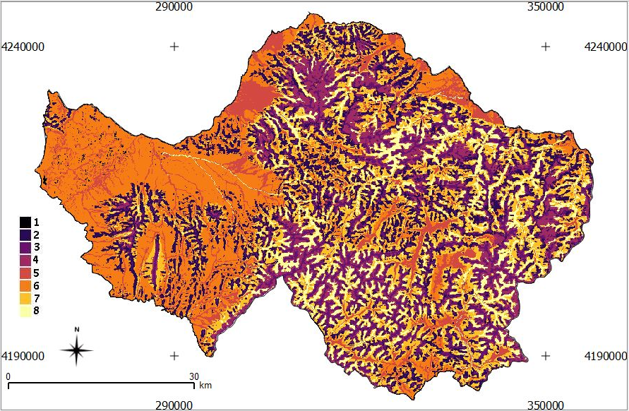
Figure 4. The spatial extent f the 8 clusters (terrain classes).
Table 2. The cluster centroids and occurrence (percent spatial extent) for the 8 cluster . Note that while in clustering the data was normalized per terrain attribute, in the current centroid presentation the actual value range per terrain attribute is presented for it’s 8 centroid co-ordinates
|
Terrain attributes |
Clusters |
|||||||
|
1 |
2 |
3 |
4 |
5 |
6 |
7 |
8 |
|
|
CND |
2.13 |
3.11 |
2.76 |
2.78 |
1.55 |
2.16 |
3.20 |
8.14 |
|
ProfC |
210.0 |
491.5 |
454.2 |
14.9 |
34.8 |
143.3 |
177.9 |
0.1 |
|
Lsf |
0.000299 |
0.001444 |
0.000353 |
-0.000311 |
-0.000108 |
-0.000634 |
-0.001104 |
-0.001255 |
|
VD |
4.3 |
5.8 |
8.8 |
1.4 |
1.2 |
6.6 |
10.8 |
5.8 |
|
DC |
61.1 |
39.4 |
107.0 |
277.2 |
108.1 |
174.6 |
284.6 |
245.3 |
|
CI |
-0.0247 |
0.2249 |
-0.2934 |
-0.1677 |
-0.0957 |
-0.3339 |
-0.7854 |
-0.6747 |
|
FPL |
6.0 |
13.2 |
0.8 |
-11.0 |
0.6 |
-1.9 |
-9.4 |
-24.1 |
|
PlanC |
2090 |
3247 |
4369 |
1081 |
991 |
1871 |
2450 |
293 |
|
PO |
0.000579 |
0.001709 |
0.000231 |
-0.000311 |
-0.000009 |
-0.000263 |
-0.001328 |
-0.000820 |
|
TWI |
1.457 |
1.469 |
1.375 |
1.464 |
1.506 |
1.370 |
1.275 |
1.353 |
|
TCA |
6.317 |
5.503 |
6.609 |
13.195 |
9.064 |
7.571 |
8.941 |
18.314 |
|
MBI |
27624 |
17317 |
62207 |
5596135 |
132949 |
137054 |
1866839 |
144024360 |
|
UC |
0.1247 |
0.2666 |
-0.0415 |
-0.0499 |
-0.0086 |
-0.0632 |
-0.2140 |
-0.1850 |
|
Occurrence |
18.47 |
8.01 |
11.94 |
9.31 |
22.65 |
20.37 |
8.87 |
0.38 |
LANDSLIDE RISK ASSESSMENT
The landslide occurrence per terrain class is computed in Figure 5 and in Table 3. According to Table 3 and Figure 5, landslides occur only in 3 terrain classes that corresponds to class 1, class 6 and class 7. The percent of landslide points (Table 3) ithin a terrain class divided by the occurrence of the terrain class (Table 2 ) is used to define the Landslide Risk Index (LRI) in Table 3.
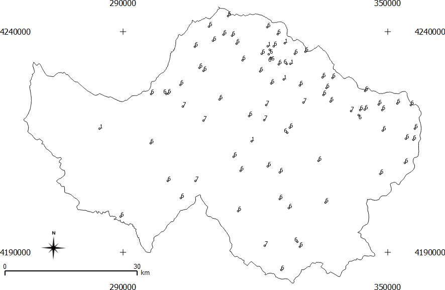
Figure 5. The landslides labeled by the terrain class they belong to.
Table 3. Landslide occurrence per terrain class.
|
Terrain class |
Number of points |
Percent of points % |
Terrain class occurrence |
Landslide risk index (LRI) |
|
1 |
6 |
7,3 |
18.5 |
0,4 |
|
6 |
68 |
82,9 |
20.4 |
4,1 |
|
7 |
8 |
9,8 |
8.9 |
1,1 |
|
Total |
82 |
100 |
47.9 |
|
Under this definition, terrain class 6 presents LRI that is almost 4 times greater than the LRI of terrain class 7 while terrain class 7 presents LRI that is almost 3 times greater than the LRI of terrain class 1. These three terrain classes are represented with standardized (in the interval 0 to 1) centroids co-ordinates in Figure 6.
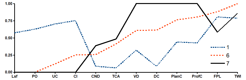
Figure 6. The standardized cluster centroids (in the interval 0 to 1) for the terrain classes 1, 6 and 7. Note than only Lsf, PO, UC, CI, CND, TCA, VD, DC, PlanC, ProfC, FPL, TWI were used in this presentation.
Profile and planar curvature (shape indices) as well as valley depth that is correlated to terraib variability within a kernel) are fixed kernel geomorphometric parameters while the rest 10 are extended neighborhood geomorphometric parameters. These parameters present a minimum correlation in between them and that is why they were selected among others under a trial and error procedure.
The compiled landslide data is very unlikely to be complete, since most landslides records are either failures of man-made or natural terrain landslides that lead to death, injury, or interruption of human activities. So for non-damaging natural terrain landslides, the location of their occurrence must be close to human activities, to catch the attention otherwise will not be reported. On the other hand, the new landslide records might be easily incorporated to the analysis since only the landslide occurrence per terrain class might be modified and not the terrain class occurrence within the study area.
In the present study the 3 arc seconds SRTM DEM data (at 100 m spatial resolution approximately) are used while 1 are second SRTM elevation data ((at 30 m spatial resolution approximately) is also available for the study area. In a future research effort, the higher spatial resolution SRTM elevation data will be used in an attempt to recompute the geomorphometric data and segment terrain classes at finer resolution/scale.
A fundamental assumption is that each terrain class is represented by the centroid vector and it’s spatial extent. So the landslide risk is considered constant in each terrain class. This is an abstraction, that is reliable for the moderate resolution DEM data (at 100 m spacing) used in this research effort. In future research efforts, variable LRI will be computed within each terrain class on the basis of higher spatial resolution DEM data.
Figure 6 indicates the variability of the standardized centroid co-ordinates for the 3 terrain classes presenting LRI > 0. Figure 6 reveals differences (for example the variability in VD, TEI, etc. etc.) in the spatial position of the three terrain classes. For example according to Figure 6, a terrain class should be closer to the river network that the others. The spatial arrangement of the 3 classes is verified more clearly in Figure 7 and Figure 8.
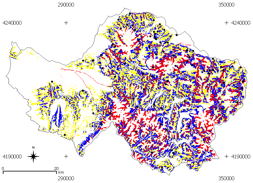
Figure 7. The terrain classes 1 (depicted in yellow), 6 (depicted in blue) and 7 (depicted in red) as well as the landslide points.
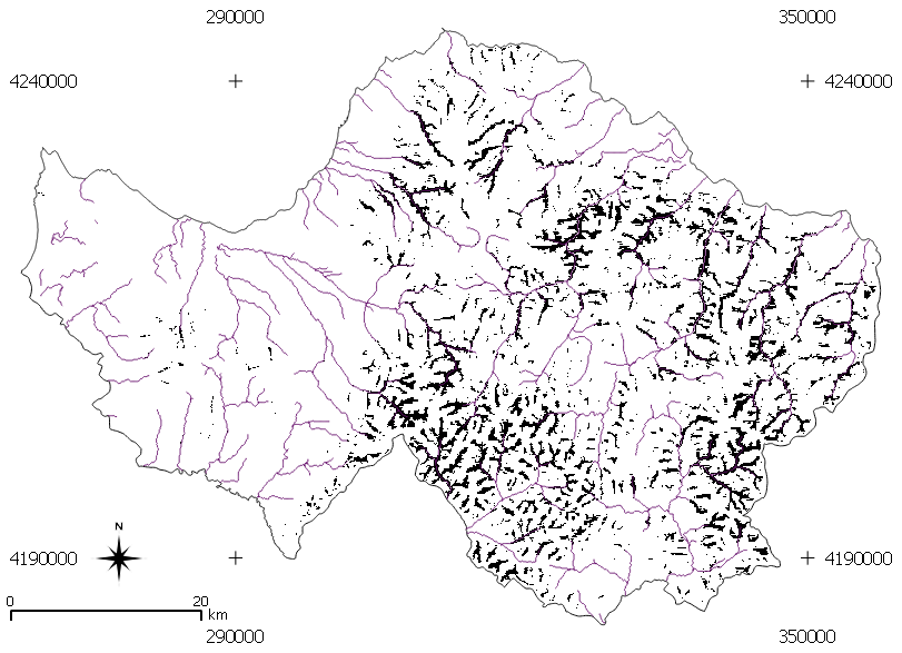
Figure 8. The river network and the terrain class 7.
The terrain segmentation on the basis of extended neighborhood and shape terrain attributes seems to be particularly useful for defining terrain classes that can be used in order to define landslide risk from point landslide data from a moderate resolution (100 m) DEM.
The percent landslide occurrence within the percent area occupied by each terrain class, is used to define a new landslide risk index (LRI) that is useful for hazard/risk assessment, landuse and landcover studies as well as rural and urban planning within the study area.
AUTHOR CONTRIBUTION
Both authors contributed to the idea, the processing and the design of the content,
Aspinall D, Rabe N, McDonald I (2015) Understanding precision agriculture: Mapping Elevation and Topographic Modelling. Ontario Grain Farmer Magazine.
Ballerine C (2017) Topographic Wetness Index. University of Illinois Urbana-Champaign.
View ArticleBoehner J, Selige T (2006) Spatial Prediction of Soil Attributes Using Terrain Analysis and Climate Regionalisation In: Boehner J, McCloy K R, Strobl J: 'SAGA - Analysis and Modelling Applications', Goettinger Geographische Abhandlungen 115:13-27.
Chau K, Sze Y, Fung M, Wong W, Fong E, Chan L (2004) Landslide hazard analysis for Hong Kong using landslide inventory and GIS: Computers & Geosciences 30:429-443.
View ArticleCostanzo D, Chacón J, Conoscenti C, Irigaray C, Rotigliano E (2014) Forward logistic regression for earth-flow landslide susceptibility assessment in the Platani river basin (southern Sicily, Italy). Landslides 11:639–653.
View ArticleDai F C, Lee C F (2002) Landslide characteristics and slope instabilitymodeling using GIS, Lantau Island, Hong Kong. Geomorphology 42:213–228. 00087-3
View ArticleDhakal A, Amada T, Anuya M (2000) Landslide hazard mapping and its evaluation using GIS, an investigation of sampling schemes for a grid-cell based qualitative method: Photogrammetric Engineering & Remote Sensing 66:981-989.
Farr TG, Kobrick M (2000) Shuttle radar topography mission produces anwealth of data. Am Geophys Union Eos 81:583–585.
View ArticleFreeman G T (1991) Calculating catchment area with divergent flow based on a regular grid. Computers and Geosciences 17:413-422. 90048-I
View ArticleGao L, Zhang L M, Chen H X (2015) Likely scenarios of natural terrain shallow slope failures on Hong Kong Island under extreme storms. Natural Hazards Review ASCE:B4015001.
View ArticleLandam S, Everitt S B (2004) A Handbook for statistical analyses using SPSS. Chapman and Hall/CRC Press, New York.
Mather P M, Koch M (2011) Computer processing of remotely-sensed images (4rd edn). John Wiley & Sons, Chichester.
View ArticleMärker M, Hochschild V, Maca V, Vilímek V (2016) Stochastic assessment of landslides and debris flows in the Jemma basin, Blue Nile, Central Ethiopia. Geografia Fisica e Dinamica Quaternaria. 39:51-58:DOI 10.4461/GFDQ 2014.39.5.
Miliaresis G (2006) Geomorphometric mapping of Asia Minor from GLOBE digital elevation model. Geografiska Annaler Series A: Physical Geography 88(3):209-221.
View ArticleMiliaresis G, Paraschou Ch (2005) Vertical accuracy of the SRTM DTED Level 1 of Crete. Int. J. of Applied Earth Observation & GeoInformation 7(1):49-59. DOI:10.1016/j.jag.2004.12.001.
View ArticleMiliaresis G, Sabatakakis N, Koukis G (2005) Terrain pattern recognition & spatial decision for regional slope stability studies. Natural Resources Research 14(2):91-100. DOI: 10.1007/s11053-005-6951-3.
View ArticleMöller M, Volk M, Friedrich K, Lymburner L (2008) Placing soil genesis and transport processes into a landscape context: A multi-scale terrain analysis approach. Journal of Plant Nutrition and Soil Science 171:419-430.
View ArticleMugnier C (2002) Grids & datum: the Hellenic Republic. Photogrammetric Engineering & Remote Sensing 68:1237-38.
NGGF (2018) Geo-database of Ground Failures. Institute for Geology and Mineral Exploration (IGME) of Greece.
View ArticlePandey S (1987) Principles & applications of photogeology: John Wiley & Sons, New Delhi.
Pike R J, Evans I S, Hengl T (2008) Geomorphometry: A brief guide. In: T. Hengl and H. Reuter, Elsevier Eds. Geomorphometry: Concepts, Software, Applications. Developments in Soil Science. Amsterdam 33:03-30.
Poyiadji E (2007) IGME Landslide Database and a Review of Hazard Zonation in Greece. Europen Soil Data Center, JRC, European Commission.
SRTM DEM (2017) Shuttle Radar Topography Mission Digital Elevation Data. US Geological Survey. .
View ArticleQin C, Zhu A, Li B, Pei T, Zhou C, Shi X (2009) Quantification of spatial gradation of slope positions. Geomorphology 110(3-4):152-161.
View ArticleRenard K G, Foster G R, Weesies G A, McCool D K, Yoder D C (1997) Predicting soil erosion by water: A guide to conservation planning with the Revised Universal Soil Loss Equation (RUSLE). Agriculture Handbook 703:384.
Sangar S, Kanungo D (2004) An integrated approach for landslide susceptibility mapping using remote sensing and GIS. Photogrammetric Engineering & Remote Sensing 70:617-625.
View ArticleShary P A (1995) Land surface in gravity points classification by a complete system of curvatures. Mathematical Geology 27(3):373–390.
View ArticleShirzadi A, Bui D, Pham B, Solaimani K (2017) Shallow landslide susceptibility assessment using a novel hybrid intelligence approach. Environmental Earth Science 76:60.
View ArticleYokoyama R, Shirasawa M, Pike R J (2002) Visualizing topography by openness: A new application of image processing to digital elevation models. Photogrammetric Engineering and Remote Sensing 68:251-266.
Zevenbergen L W, Thorne C R (1987) Quantitative Analysis of Land Surface Topography. Earth Surface Processes and Landforms 12:47-56.
View Article