Watershed Modeling and Sediment Yield Prediction of the Los Olmos Creek Watershed in South Texas

Jungseok Ho and Chu-Lin Cheng

chulin.cheng@.utrgv.edu; jungseok.ho@utrgv.edu

Rockford Miller^1,3, Jungseok Ho¹ and Chu-Lin Cheng^1,2

¹ Department of Civil Engineering, University of Texas – Rio Grande Valley

² School of Earth, Environmental and Marine Sciences, University of Texas – Rio Grande Valley

³ PSI Corporate Consultant, Harlingen, TX

Chu-Lin Cheng, Watershed Modeling and Sediment Yield Prediction of the Los Olmos Creek Watershed in South Texas(-0001)SDRP Journal of Earth Sciences & Environmental Studies 1(1)

Studying the sediment that accumulates in a stream is an important aspect in the study of water quality and resources. With respect to water quality, the main issue is the turbidity of the water. Increased losses of natural landscape increase the erosion process in turn raising the turbidity of the water and reducing the light that can penetrate to the water reducing the growth of aquatic life. With respect to water resources, sediment accumulates in the river ways, harbors, and in dams reducing the effectiveness of these resources. This study focused on determining the amount of sediment that is outputted at the outlet of a watershed in the form of sediment yield in units of Tonne per square kilometer.
The objective of this study was to determine and produce a map that detailed the sediment yield in Tonne per square kilometer for the subbasins within the Los Olmos Creek watershed given a hypothetical frequency storm event. Two frequency storm events were applied and compared and the final outcome would be sediment yield per storm event.

Studying the sediment that accumulates in a stream is an important aspect in the study of water quality and resources. With respect to water quality, the main issue is the turbidity of the water. Increased losses of natural landscape increase the erosion process in turn raising the turbidity of the water and reducing the light that can penetrate to the water reducing the growth of aquatic life. With respect to water resources, sediment accumulates in the river ways, harbors, and in dams reducing the effectiveness of these resources. This study focused on determining the amount of sediment that is outputted at the outlet of a watershed in the form of sediment yield in units of Tonne per square kilometer. 

The objective of this study was to determine and produce a map that detailed the sediment yield in Tonne per square kilometer for the subbasins within the Los Olmos Creek watershed given a hypothetical frequency storm event. Two frequency storm events were applied and compared and the final outcome would be sediment yield per storm event.

After determining the parameters of the study, an investigation into the parameters required. The modified universal soil loss equation was first developed by Jimmy R Williams in 1975. The factor that makes it different from the universal soil loss equation is the fact that it takes in account into the energy that is associated with runoff due to the fact that this is the main driving force of erosion via water. The energy from the runoff is due to the volume of water is flowing off the watershed and the peak flow rate, which was discussed Sediment Yield Predictions with Universal Equation Using Runoff Energy Factor (Williams, 1975). Prediction of Sediment Yield Plains Grasslands with the Modified Universal Soil Loss Equation, written by Smith et. al. (1984). This paper is application and case study of the MUSLE developed by Williams (1975) and applied to grassland regions of Texas and Oklahoma that consists of animal grazing lands and cultivation of rowed crops. The study was able to determine the sediment yield per storm event using the MUSLE and predicted values. Then compare the data derived from the MUSLE using field data. The comparison showed a strong correlation of predicted values versus field data values. Another paper that was looked into was titled The Dimensional Analysis of the USLE-MUSLE Soil Erosion Model, written by Petru Cardei (2010). This paper outlines multiple techniques in which one can determine empirically, the rainfall erosivity factor and runoff energy factor, and then the general sediment yield. The places multiple components in a dimensional analysis environment pillow for ways to improve upon each of the equations so that more of a simplistic form can be derive for quicker computation. Applicability of the Modified Universal Soil Loss Equation for Prediction of Sediment Yield in Khanmirirza Watershed, Iran, was written byS.H.R Sadeghi and T. Mizuyama and details a case example an application of the MUSLE. The study included field data and monitoring during six storm events and demonstrated the effectiveness of the MUSLE. Sediment and Erosion Design Guide, developed by Mussetter Engineering Inc. and stamped by Professional Engineer, Mussetter (2008). The design guide covers a wide range of sediment and erosion details in particular the focus was on the utilization of the MUSLE. Streamflow Analysis using ArcGIS and HEC GeoHMS was written by Han (2010). The paper was about the application of GeoHMS within ArcGIS and then using the data created with GeoHMS in HMS for streamflow analysis. A GIS-based Hydraulic Bulking Factor Map for New Mexico was written by Gallegos et. al (2014). This paper utilized ArcGIS, HEC GeoHMS and HEC HMS and developed a bulking factor map or sediment load map for the 8 small watersheds within the state of New Mexico. It focuses on sediment loading with respect to water channeling and sediment buildup. Sediment and its Effect on Water Quality written by Elliott Flaxman. This paper details the impact of sediment and water quality. It details many uses of water, for example, recreation, industrials and agricultural and how the sediment effect each of the categories.

1. Watershed

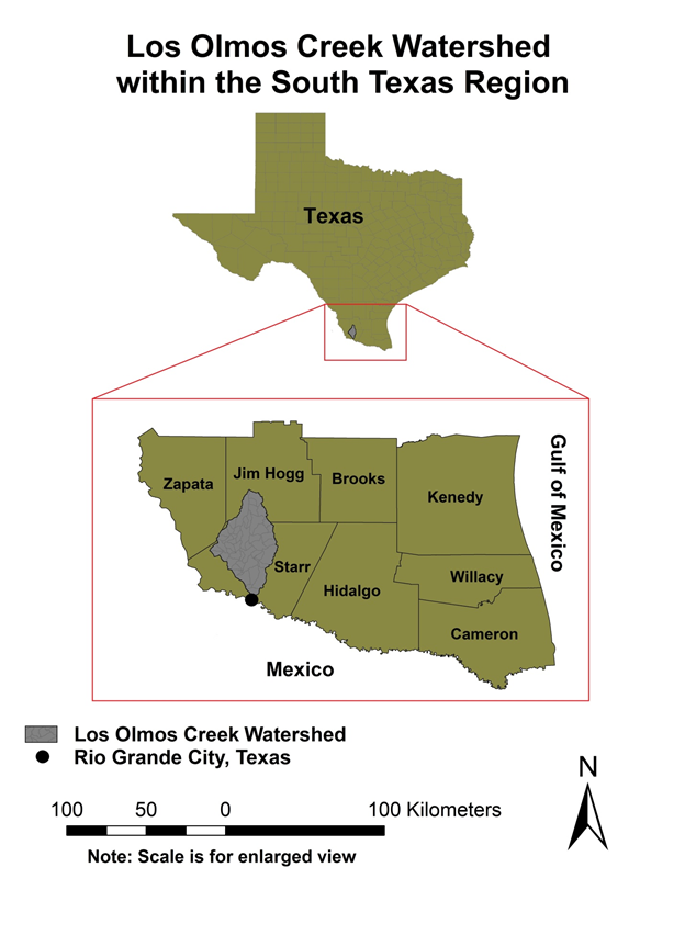
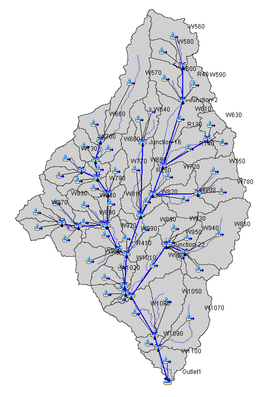
The watershed that was examined in this study was the Los Olmos Creek Watershed, the mouth of which is located in the Rio Grande City, Texas. The watershed is approximately 1369 square kilometers and is the only isolated watershed below Falcon Dam located on the north side of the Rio Grande River. A map of the watershed can be seen at Figure 1. This study utilized the Hydrologic Engineering Center Geospatial Hydrologic Modeling Extension (HEC GeoHMS) tool kit within ArcGIS; then applied what was created in ArcGIS with the GeoHMS tool kit and inserted the data into Hydrologic Engineering Center Hydrologic Modeling System (HEC HMS) for hydrologic analysis. HEC HMS has a function called Sediment Erosion Module that calculates the sediment yield of a watershed using the Modified Universal Soil Loss Equation (MUSLE). Other data that need to gathered and processed for the study included the utilization of ArcGIS alone and the data processed with spreadsheet applications and then inserted into HEC HMS. The MUSLE is explained as follows:

SY = (α·(Q·q_n)^0.56 )·K·LS·C·P                                                              Equation 1

where, SY = sediment yield in tonne/km², α = regional coefficient, Q = runoff volume in m³, q_n = peak flow rate in m³/sec, K = erodibility factor, LS = topographic factor, C = cover and management factor, P = land conservation factor.

Data

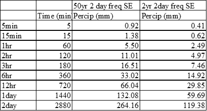
 The Digital Elevation Map (DEM) and National Hydrologic Dataset (NHD) from the United States Geological Survey were necessary for the development of the watershed subbasins for analysis with HEC HMS. Soil data was retrieved from Gridded Soil Survey Geographic data (gSSURGO) and the land coverage data was from the National Land Coverage Dataset (NLCD) 2011, both of which came from the Geospatial Data Gateway through the National Resources Conservation Service (NRCS). Precipitation and frequency storm event data were from the US Department of Commerce, Weather Bureau, Technical Paper No. 49. Gradation data was based on the 0.45 Power Maximum Density Curve, developed by the Federal Highway Administration using the maximum aggregate size of 19mm.

Data collection

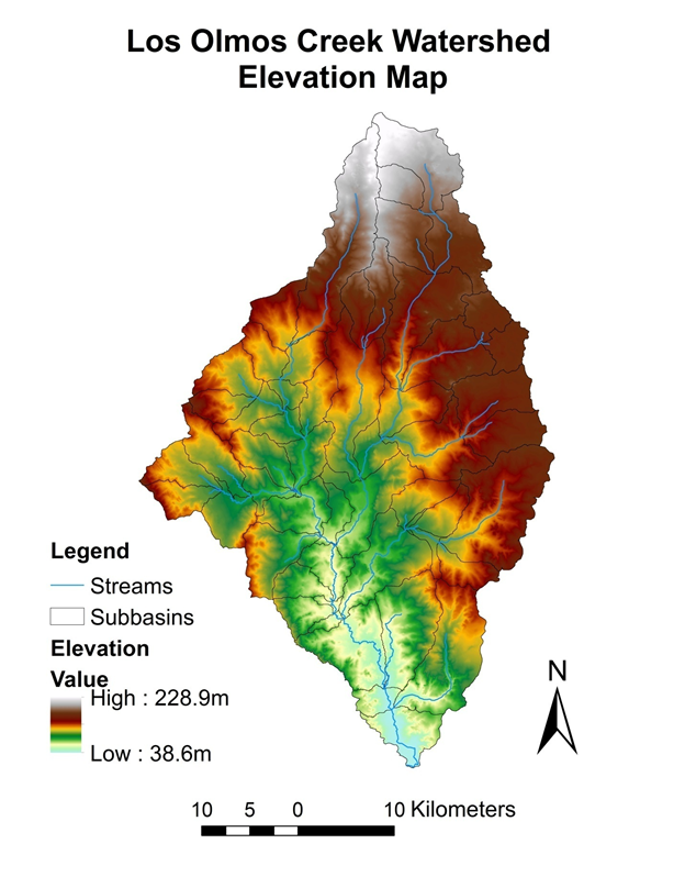
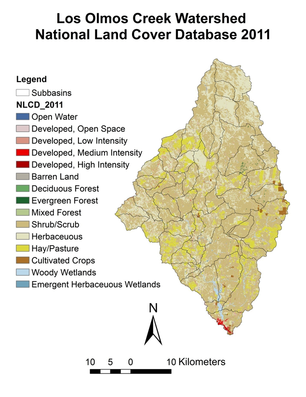
The data that was initially required for processing inside ArcGIS for preparation for GeoHMS was a digital elevation map (DEM) of the subject site as well as National Hydrologic Dataset (NHD), of the latter the most important for determining the shapefile of the Los Olmos Creek watershed which consisted of four subbasin10-HUC as well as the flow lines that represents the streams of the watershed. The DEM and NHD were retrieved from the United States Geological Survey (USGS) website National Map Viewer. First the manipulation of the DEM was required. This required two different raster files that had to be mosaic/merged together through the raster mosaic toolkit. The DEM’s for the study area were high-resolution 10 meter raster files. After the raster’s are merged together, the shapefile of the Los Olmos Creek watershed was overlaid on top of the merge DEM’s. An extraction by mask was executed revealing only the DEM of the watershed. The in NHD flow lines were then overlaid on top of the watershed shapefile and simply clipped to only include the flow lines within the watershed. At this point, the process of preprocessing within GeoHMS was ready to initiate. Before this GeoHMS was started other data was collected for the project; this included gridded SSURGO data which included soil data for the entire state of Texas as well as the National Land Use Dataset for the entire state of Texas. An elevation map of the watershed and the NLCD 2011 watershed map can be seen on Figures 2 and 3, respectively.

 Coordinates

This is an important part of the project and ensured accurate measurements and spatial referencing. For this project I continuously tried to set my coordinates for the data frame in a Albers equal area projection USGS, North American Datum 1983 (NAD 83), US foot unit linear measurement, to include all maps. This projection was recommended by the GeoHMS manual or maintaining the dimensional integrity of the watershed during watershed delineation. I specified that I continuously tried as I was unsuccessful in projecting the data frame and map layers. Instead I maintained the data frame non-projected on a coordinate system of Geographic Coordinate System, NAD 83 and all layers were projected with respect to the Albers equal area projection USGS, NAD 83, meter at the linear unit of measurement. For some reason or another I couldn’t complete the GeoHMS preprocessing with US foot linear unit of measurement. Research indicates that it could be a AP framework malfunction within the source code of ArcGIS.

 HEC GeoHMS

 GeoHMS preprocessing

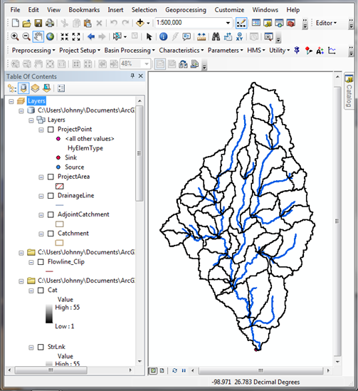
After the DEM and the stream flow lines were gathered and everything fit within the watershed the process of preprocessing the data for implementation inside a GeoHMS could proceed. This process is essentially watershed delineation and created a series of raster maps that follow a particular order during the creation process. It is important to ensure that each step is followed and it is in proper order. The first step was to execute a DEM reconditioning which involved the original DEM as well as the in NHD flow lines of the watershed. The DEM reconditioning tool was open and these two elements were attached to function and executed. This function allows for a better spatial referencing with respect to the DEM low points, valleys and existing in NHD flow lines. The next function was to fill the sinks within the reconditioned DEM. This essentially created a depression less DEM that helps to mitigate problems that will arise during future watershed delineation and analysis. The next step in the preprocessing phase was to determine flow directions. This function essentially determined the aspect of the topography to determine which direction water will flow. The function only required the fill raster. The next phase was determining the flow accumulation, essentially where water would accumulate during a storm event. As logic would follow the flow accumulation map highlighted the areas of the rivers and streams locations and continue to help better define the streams and topography of the DEM. Next phase was stream segmentation, this essentially created segment of the linked streams that was from the flow accumulation map. The next raster file was the stream segmentation linkage function, which took all the stream segments and linked them together to create streams throughout the watershed. After this phase we now have an accurate approximation of the streams with respect to the DEM. The next phase was to create catchment polygons throughout the DEM. These would essentially be the predecessors of the future subbasins in the HMS map. The function essentially breaks up the watershed and creates a shapefile within GeoHMS database for implementation of attribute tables and other relevant data. Breaking the watershed into subbasins allows for better watershed analysis for particular regions within the watershed. After the catchment polygons were created a process of refining the catchment polygons, then drainage lines attachment and finally adjoinment of the catchment polygons with respect to the drainage lines could be determined for final shapefile as shown in Figure 4.

GeoHMS Project Setup

After the preprocessing of the watershed was complete the resulting shapefile could be moved over and prepared for a project creation within GeoHMS. One just starts a new project by selecting new project inputting the data for example project name identifying project points and area and set in new threshold parameters for the project which was the accumulated cells of the project. After the project was created you can establish the outlet of the watershed which for my case was at the southernmost tip of the watershed. After the outlet was established the project could be generated. This essentially created all the attribute tables and parameters that were going to be executed and filled out later during the GeoHMS process. After the project was generated a required confirmation of the project area was necessary and close detail needs be paid attention to ensure that the area encompasses the entire watershed.

Geo HMS Basin Processing

For this particular study basin merging or basin dividing was not required. However, there is the function within the basin processing that allows for double checking of streams within particular subbasins, called river merge. Working through the each subbasin and ensuring that each river segment is connected throughout the subbasin.

Geo HMS Characteristics

Developing the watershed characteristics first required establishing River length and river slope of the watershed. Next was to develop the basin slope this was the average slope for each subbasin. In order to fully execute this task Arc Hydro Tools was necessary and the slope tool under terrain preprocessing. This tool utilize the percent slope of the watershed. After a raster of the watershed with respect to slope percent the basin slope tool can be used in a Geo HMS this computer the average basin slope for each subbasin. Next was developing the longest flow path for each subbasin this function utilized all the preprocessing data and was able to determine at which point within each subbasin the flow would accumulate from the very beginning of the subbasins. Next was to determine the basin centroid. This function essentially established geometric center of each subbasin was located. After establishing each subbasins centroid the centroid elevation to establish with the DEM raster. Another function within the characteristics was the central centroid rule longest flow path this was just determining from the centroid to the outlet of the subbasin. This last function concluded to watershed characteristics.

GeoHMS Parameters

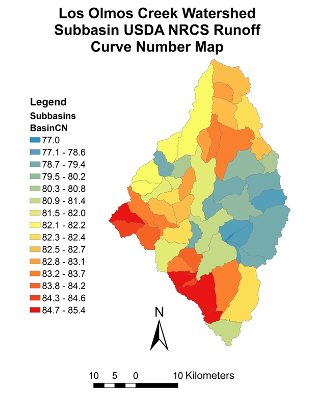
            The next phase was establishing the parameters for the HMS model. The first step was to establish and select HMS processes this included identifying loss method for initial abstraction, transform method for unit hydrograph, and baseflow method and river route method. The loss method and base flow method were excluded from this study. The transform method used for the unit hydrograph was the Soil Conservation Service (SCS) NRCS unit hydrograph. For the river route method the SCS lag method was utilized. The next set of functions within parameters included the automatic naming of the river and subbasins within the watershed for easier identification in HMS modeling. Subbasin parameters from raster and subbasin parameters from features includes a function where you can insert raster and shape file mass respectively that utilizes a zonal statistical tool to determine averages for subbasins. For the subbasin parameters from raster the only parameters that were utilize were the percentage of impervious grid surfaces and the input curve number grid that was developed outside GeoHMS. No parameters were utilized for the subbasin parameters from features. The last thing that was utilized in the parameters function was a generation of the CN lag. The CN lag populates the basin CN and basin slope columns in the subbasins attributes table. None of the TR 55 parameters were utilized in this study due to the fact that the raster file that was needed for this function was not available through the National Oceanic and Atmospheric Administration (NOAA) due to being updated. The raster that was being updated was the two-year rainfall grid raster.

GeoHMS to HMS map development

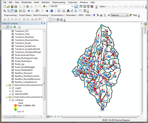
This stage of the project is where the HMS files are really starting to be established. These include updating the HMS map units, verifying that all data is correct, updating HMS schematics, and including cornets for the HMS files. The data was then prepared for export and saved to new files, a subbasin shape file was created that included the whole watershed, the subbasins within the watershed, and the streams. At this point the HMS project is ready for implementation in HMS however a couple parameters need be included. A final screens image of the GeoHMS processed watershed map can be seen on Figure 5.

Parameters That Were Not Included in GeoHMS for MUSLE

In order to determine the erodibility factor, topological factor, topographic factor and the cover and management factor one needs to create a new data set and do this without the assistance of Geo HMS.

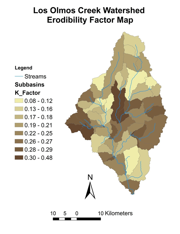
  Erodibility factor

The erodibility factor or K factor is the factor has to do with how the soil erodes. It is based upon soil type (sand, silt or clay) and organic matter content. For this study the case factor was found in gridded SSURRGO data under the table chorizon. In order to move this table over to the watershed subbasins shape file, I needed to first work in the gridded SSURRGO data, join the component table to the chorizon table with the mukey column to a raster of the watershed that contain no subbasins.. Mukey is the identification marker for the shapefiles. First I created a new field in the watershed raster titled K factor. After joining the component and horizon table with the Mukey, I can then join component to the watershed raster and the data for component and horizon was now joined to the watershed raster. I then used the field calculator and set the K factor field equal to the K factor in the horizon table, and then remove the join. This leaves me with the K factor in the watershed subbasins raster.  At this point I used the zonal statistical tool spatial analysis toolset in ArcGIS. The inputs for the zonal statistical tool acquire the target shapefile the watershed subbasins and the watershed raster with the K factor. The subbasin names were identified in the zonal statistical executed. This will take all the data from the watershed raster and determine averages all the individual subbasin leaving an average K factor for each subbasin within the watershed subbasin shapefile. The data for this can be seen on on Figure 6.

 Topographic factor

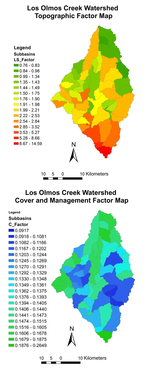
            Is factor has to do with how well the water moves on the surface of the land. Steeped short slopes will create more erosion then long flat section. The topographic factor is the multiplication of the slope length factor and slope percent factor. These maps are first generated individually with ArcGIS and then multiplied to give a topographic factor. The following maps were generated with respect to the watershed raster map. First the slope steepness factor or S factor was generated. The slope tool in the spatial analyst toolbar was used with respect to slope percent this raster would be used with the raster calculator with the following equation. After the computation of the previous equation the generated map was a slope steepness factor. Next was to determine the slope length factor or L factor. This was done with the raster calculator and the flow accumulation raster that was generated during watershed delinazation, and cell size of the flow accumulation raster. The following equation was used in the raster calculator. After both the slope steepness factor map and the slope length factor map was generated the data was inserted into the watershed raster map via the zonal statistical tool for determining the average slope length factor in slope steepness factor of each subbasin. At this point the field calculator was used to multiple the average slope length factor in slope steepness factor of each subbasin to create the average topographic factor or LS factor for each subbasin. The data for this can be seen on Table 1 and the ArcGIS generated map is at Figure 6.

Cover and Management Factor

The cover and management factor was derived from the NLCD 2011. Essentially, the cover descriptions where given a range from bare impervious surfaces being a 1 value and highly organic forest soils a value of 0.0001(Pak 2015). The descriptions in the NLCD 2011 covered a large range of surface types each type was given a particular C factor is an image of the watershed NLCD with the attributes table showing the cover descriptions and see factors. After the C factors were set the zonal statistical tool could be applied to the watershed NLCD 2011 raster map. The C factor was the category that was given the average subbasin within the watershed raster. The final map of this could be seen in Figure 7.

Practice Factor

Practice factor has to do with the agricultural row crop cultivation and since observations from the NLCD 2011 show very little agricultural road crop cultivation this factor was set to a value of 1 for computation in the MUSLE. The watershed NLCD 2011 can be seen at Figure 3.

 Implementation in HMS

 Watershed Geo HMS development and the MUSLE factors had been generated HMS was started in a new project was created. First the importation of the subbasin shapefile and streams file to create background. Components were added to the project these being Basin Model, Meteorologic Model, Control Specifications and Paired Data. After components of establish the parameters for the components were inserted. The simulation runs was created for each storm event

 Basin Model

            The basin model contains all of the elements of the watershed. The elements include precipitation gauges in each subbasin, reaches, junctions and the outlet. When importing basin file from Geo HMS each subbasin had a reach downstream to the outlet, this needed to be corrected injunctions inserted where necessary. Figure 9 shows the sub-basins of the watershed.

Meteorologic Model

            Two frequency storm events were derived from US Department of Commerce weather Bureau technical paper No. 49. A 50 year 2 day precipitation average for the area of the Los Olmos Creek watershed showed a precipitation level of 10.4 inches. For the 2 year 2 day precipitation the average was 4.7 inches. These values were converted to millimeters and inserted in the frequency storm precipitation column with duration.

Control Specifications

            The control specifications are the time parameters for the simulation run. For each the frequency storm events, a 14 day duration was utilized.

 Paired Data

            Paired data is the area in which holds the gradation information for computing the MUSLE. Diameter-Percentage function was the method which gradation information was used. This study utilized the Federal Highway Administration’s 0.45 Power Maximum Density Curve with a maximum aggregate size of 19 mm. The data that was inserted was of two columns, one of the diameters of aggregate and the other percent finer material.

Parameters

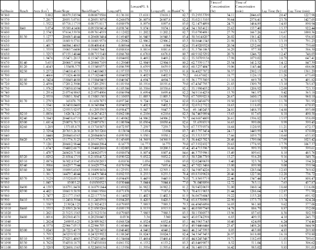
After the components were established the parameters could be inserted. For the transform method SCS method was used this required the lag time for each subbasin which was computed with respect to time a concentration. First, the time of concentration had to be computed for each subbasin. The following equation was used:

t_c = L^0.8*        (s¹ +25.4)^0.7/4238+S^0.5                                                                         Equation 2

where, t_c = the time of concentration, L = the flow length (m), CN = the NRCS Curve Number, S = 25400/CN – 254, the average slope of the subbasin in percent.

After the time a concentration was computed the lag time was calculated with the following relationship: t_L = 0.6t_c, where t_L = the lag time. Next the erosion parameters were inserted with respect to the MUSLE. This was where the erodibility factor, topographic factor, cover and management factor and gradation information was identified and utilized. Next the river routing information was inputted, for this the lag method was used. The lag method required the lag time for each reach within the subbasins. First the subbasin with respect to the reach was identified and that lag time from the subbasin was used to the corresponding reach. All data tables with respect to the parameters can be observed Tables 2 and 3.

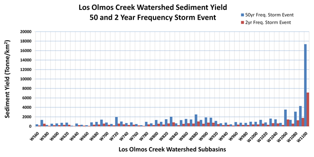
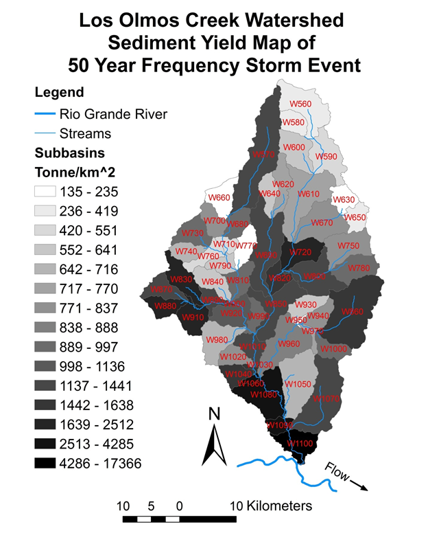
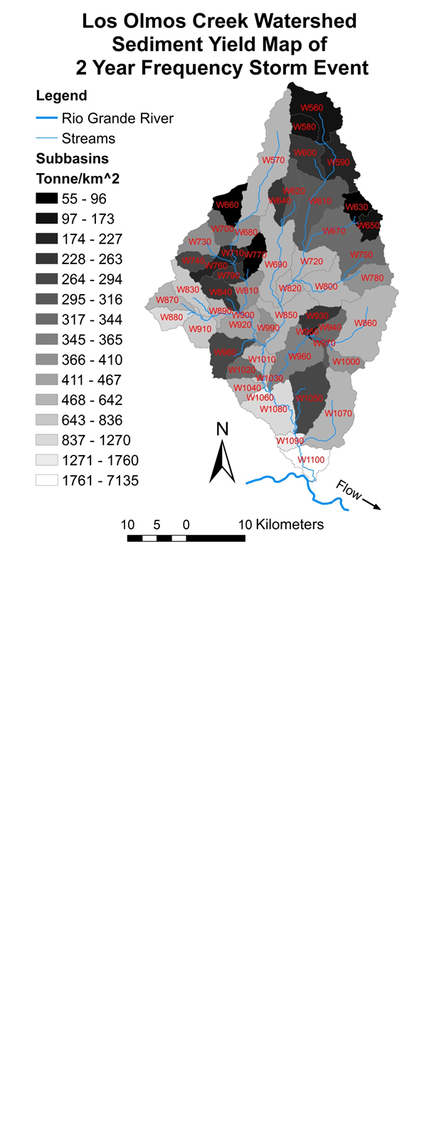
A simulation run was created for each frequency storm event. The only variation between the frequency storm events was the level of precipitation. All the other parameters stayed the same for each frequency store event. The results of the analysis with the HEC HMS Sediment Erosion Module produced the sediment load per subbasin in Tonne within the Los Olmos Creek Watershed. The sediment load was then divided by the area of the subbasin which resulted in the sediment yield, Tonne per square kilometer. The subbasins with the greatest topographic factor, greatest erodibility factor and greatest cover and management factor produced the greatest sediment yield, this being the area of the southernmost region of the watershed and the location of the outlet. The total sediment yield of the watershed during the 50 year frequency storm event yielded 78,376 Tonne per square kilometer and the 2 year frequency store event yielded 31,967 Tonne per square kilometer. Figure 10 shows the sediment yield for 50 and 2 frequency year storm events. The computed sediment yields are accumulated at the outlet. The computed sediment yield of the 50 and 2 frequency years are identified in each watershed in Figure 11 and 12, respectively. Due to the sediment transportation along the channels and deposition at the low slopped subbasin, darker colored subbains are plotted along the channels and the Arroyo Los Olmos outlets. Table 4 shows the computed sediment yields in unit of tonne/km².12:27:38

When the data was computed with HEC HMS and then imported and processed with ArcGIS and spreadsheet, the results showed that the steeper, shorter slope areas that had minimal cover yielded the greatest sediment loading. The runoff energy that was created by the precipitation moved all three types of soils classes: clays, silts and sands, however, clay, due to it particulate size was affected the most. The subbasin that was connected to the outlet, located at the southern tip of the watershed was also the subbasin of the greatest sediment yield. The combination of ArcGIS with HEC GeoHMS for watershed development and HEC HMS for watershed sediment yield analysis proved to be an effective method for approximating the sediment yield of any given watershed.

1. Cardei, Petru (2010), "The Dimensional Analysis of the USLE-MUSLE Soil Erosion Model." Proc. Rom. Acad., Series B: 249-53. Online.

2. Flaxman, Elliott (1967), "Sediment and its Effect on Water Quality" New Mexico State University, New Mexico Water Conference March 1967. Online.

3. Gallegos, J., Richardson, C., Cal, M., and Bulut, G. (2014). "GIS-Based Hydraulic Bulking Factor Map for New Mexico." J. Hydrol. Eng., 19(1), 159?166. Online. HE.1943-5584.0000727

   View Article           

4. Han, Jeongwoo (2010), "Streamflow Analysis Using ArcGIS and HEC GeoHMS." Texas A&M University, Zachry Department of Civil Engineering. Online.

5. Heath, Jared, and Johannes Beeby, (2006), "A QUALITATIVE INDEX OF SOIL EROSION FOR THE TEKEZE RIVER WATERSHED IN ETHIOPIA." Concepts in GIS - NR505. Colorado State University.

6. Mussetter Engineering Inc. (2008), "Sediment and Erosion Design Guide", Mussetter Engineering Inc.

7. National Resources Conservation Service, (2012), "Geospatial Data Gateway."Geospatial Data Gateway. National Resources Conservation Service.

8. Pak, J.H., Fleming, M., Scharffenberg, W., Gibson, S., Brauer, T., (2015), "Modeling Surface Soil Erosion and Sediment Transport Processes Using HEC HMS". United States Army Corps of Engineers.

9. Pavement Interactive (2009), "Gradation and Size." Gradation and Size. Pavement Interactive.

10. S. H. R. SADEGHI , T. MIZUYAMA (2007), "Applicability of the Modified Universal Soil Loss Equation for prediction of sediment yield in Khanmirza watershed, Iran" Hydrological Sciences Journal Vol. 52, Issue 5.

11. Smith, S. R., J. R. Williams, R. G. Menzel, and G. A. Coleman (1984), "Prediction of Sediment Yield from Southern Plains Grasslands with the Modified Universal Soil Loss Equation." Journal of Range Management 37(4): 295-97

    View Article           

12. United States Army Corps of Engineers Hydrologic Engineering Center (2014), "Geospatial Hydrologic Modeling Extension User's Manual Version 10.1", United States Army Corps of Engineers.

13. United States Army Corps of Engineers Hydrologic Engineering Center (2013), Hydrologic Modeling System User's Manual Version 4.0. United States Army Corps of Engineers.

14. United States Geological Survey (2015), "USGS TNM 2.0 Viewer." USGS TNM 2.0 Viewer. United States Geological Survey.

15. United States Geological Survey (2006), "The Impact of Sediment on the Chesapeake Bay and its Watershed" United States Geological Survey.

16. United States Department of Commerce Weather Bureau (1964), "Technical Paper No. 49, Two to Ten Day Precipitation For Return Periods of 2 to 100 Years in the Contiguous United States", United States Department of Commerce.

17. Viessman, W., and G. Lewis (2003), "Introduction to Hydrology", 5th ed. N.p.: Prentice Hall

18. Williams, Jimmy R. (1975), "Sediment Yield Predicting with the Universal Equation Using Runoff Energy Factor." Present and Prospective Technology For Predicting Sediment Yields and Sources: 244-52. United States Department of Agriculture Agricultural Research Service